Plot methods for the package's results
Source:R/hotspot.R, R/justice.R, R/plots.R, and 1 more
plot-methods.RdEvery result the package returns draws itself with plot(): no
arguments beyond the object are needed, and every method takes the same
customisation (main, col or palette, ... for
the base-graphics call, the grid from the session option; see
bricklayer_plot_options). Titles fit their panel: a title
too wide for it is drawn a step smaller, and in a panel set one that still
does not fit becomes a letter with the key printed under the panels (the
returned data carry it as the panel_key attribute); the left margin
is sized from the widest tick label, so an axis title never overlaps the
numbers. (Session defaults: see
bricklayer_plot_options for the session defaults). Each
method returns the data it drew, invisibly, as a data frame.
Usage
# S3 method for class 'rmbl_hotspot'
plot(x, ..., main = NULL, col = NULL, palette = NULL)

# S3 method for class 'rmbl_case_flow'
plot(
  x,
  ...,
  what = c("flow", "clearance"),
  main = NULL,
  col = NULL,
  palette = NULL
)

# S3 method for class 'rmbl_life_table'
plot(x, ..., main = NULL, col = NULL, palette = NULL)

# S3 method for class 'rmbl_disposition_mix'
plot(x, ..., main = NULL, col = NULL, palette = NULL)

# S3 method for class 'rmbl_density'
plot(x, ..., points = TRUE, main = NULL,
  col = NULL, palette = NULL)

# S3 method for class 'rmbl_knox'
plot(x, ..., main = NULL, col = NULL, palette = NULL)

# S3 method for class 'rmbl_clearance_decomposition'
plot(x, ..., what = NULL,
  max_parts = 20L, main = NULL, col = NULL, palette = NULL)

# S3 method for class 'rmbl_stock_flow'
plot(
  x,
  ...,
  what = c("adp", "alos", "people", "days"),
  main = NULL,
  col = NULL,
  palette = NULL
)

# S3 method for class 'rmbl_yoy'
plot(
  x,
  ...,
  what = c("pct_change", "value"),
  main = NULL,
  col = NULL,
  palette = NULL
)

# S3 method for class 'rmbl_rate'
plot(x, ..., period = NULL, main = NULL, col = NULL, palette = NULL)

# S3 method for class 'rmbl_share'
plot(x, ..., main = NULL, col = NULL, palette = NULL)

# S3 method for class 'rmbl_rate_change'
plot(x, ..., main = NULL, col = NULL, palette = NULL)

# S3 method for class 'rmbl_band_sensitivity'
plot(x, ..., main = NULL, col = NULL, palette = NULL)

# S3 method for class 'rmbl_drift_calibration'
plot(x, ..., main = NULL, col = NULL, palette = NULL)

# S3 method for class 'bricklayer_drift'
plot(x, ..., main = NULL, col = NULL, palette = NULL)

# S3 method for class 'bricklayer_benford'
plot(x, ..., main = NULL, col = NULL, palette = NULL)

# S3 method for class 'bricklayer_power'
plot(x, ..., main = NULL, col = NULL, palette = NULL)

# S3 method for class 'bricklayer_freq'
plot(x, ..., main = NULL, col = NULL, palette = NULL)

# S3 method for class 'bricklayer_missingness'
plot(x, ..., main = NULL, col = NULL, palette = NULL)

# S3 method for class 'rmbl_region_coverage'
plot(x, ..., main = NULL, col = NULL, palette = NULL)

# S3 method for class 'bricklayer_outliers'
plot(x, ..., main = NULL, col = NULL, palette = NULL)

# S3 method for class 'bricklayer_correlations'
plot(x, ..., main = NULL, col = NULL, palette = NULL)

# S3 method for class 'bricklayer_cortable'
plot(x, ..., main = NULL, col = NULL, palette = NULL)

# S3 method for class 'bricklayer_falsification'
plot(x, ..., main = NULL, col = NULL, palette = NULL)

# S3 method for class 'rmbl_bounds'
plot(x, ..., main = NULL, col = NULL, palette = NULL)

# S3 method for class 'rmbl_crf'
plot(x, ..., exposure = NULL, main = NULL, col = NULL, palette = NULL)

# S3 method for class 'rmbl_burden'
plot(x, ..., main = NULL, col = NULL, palette = NULL)

# S3 method for class 'rmbl_equity'
plot(x, ..., main = NULL, col = NULL, palette = NULL)

# S3 method for class 'rmbl_pollution_report'
plot(x, ..., main = NULL, col = NULL, palette = NULL)

# S3 method for class 'rmbl_footprint'
plot(x, ..., main = NULL, col = NULL, palette = NULL)

# S3 method for class 'rmbl_field'
plot(x, ..., contours = 8L, main = NULL, col = NULL, palette = NULL)

# S3 method for class 'rmbl_particles'
plot(x, ..., main = NULL, col = NULL, palette = NULL)

# S3 method for class 'rmbl_count_trend'
plot(x, ..., main = NULL, col = NULL, palette = NULL)

# S3 method for class 'bricklayer_analysis'
plot(x, ..., which = NULL, main = NULL)

# S3 method for class 'rmbl_svy_estimate'
plot(x, ..., main = NULL, col = NULL, palette = NULL)

# S3 method for class 'rmbl_svy_compare'
plot(x, ..., main = NULL, col = NULL, palette = NULL)
Arguments
- x
The result.
- ...
Passed to the base-graphics call (
plot,barplotorimage); forbricklayer_analysis, passed on to each panel's method.- main
Title; each method has a default.
- col
Colours, overriding the palette.
- palette
A
bricklayer_palettename, overriding the session option.- what
For
rmbl_stock_flow, the measures to draw (one panel each): any of"adp","alos","people","days","flow_rate","stock_rate". Forrmbl_yoy,"pct_change"or"value". Forrmbl_case_flow,"flow"and/or"clearance"; forrmbl_clearance_decomposition, any of"rates","mix"and"effects"(the default fits the device).- points
For
rmbl_density, whether to draw the incidents over the surface.- max_parts
For
rmbl_clearance_decomposition, the most parts drawn: past it, the parts that moved the aggregate most, and the rest summed into one row.- period
For
rmbl_rate, abycolumn holding the period: the rate is drawn over time with its interval band, one panel per group of the otherbycolumns.- exposure
For
rmbl_crfandrmbl_burden, the exposure range to draw the curve over; the default runs from 0 to 1.5 times the exposure in the object.- contours
Number of contour lines over a field image (0 for none).
- which
For
bricklayer_analysis, the panels: any of"change","rates","rate_change";NULLdraws every panel the analysis has.
Details
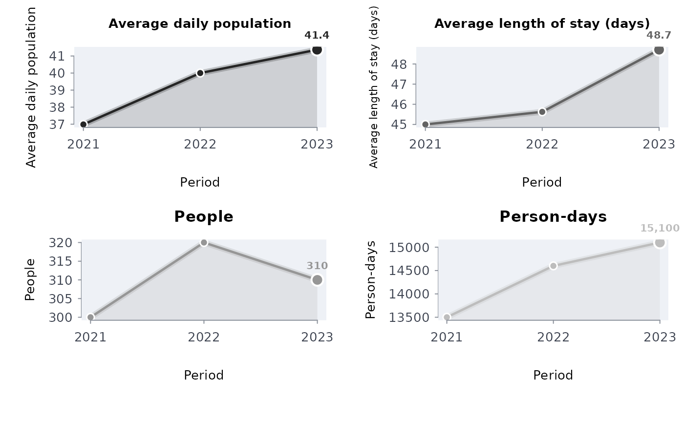
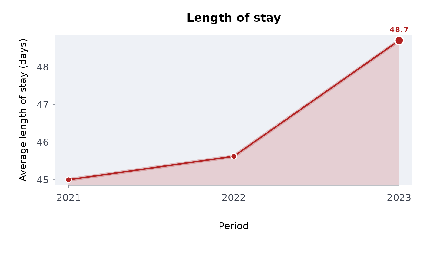
rmbl_stock_flow(
stock_flow) the average daily population, length of stay, people and person-days over the periods, one panel per measure inwhat; with an exposure, the flow and stock rates too.rmbl_yoy(
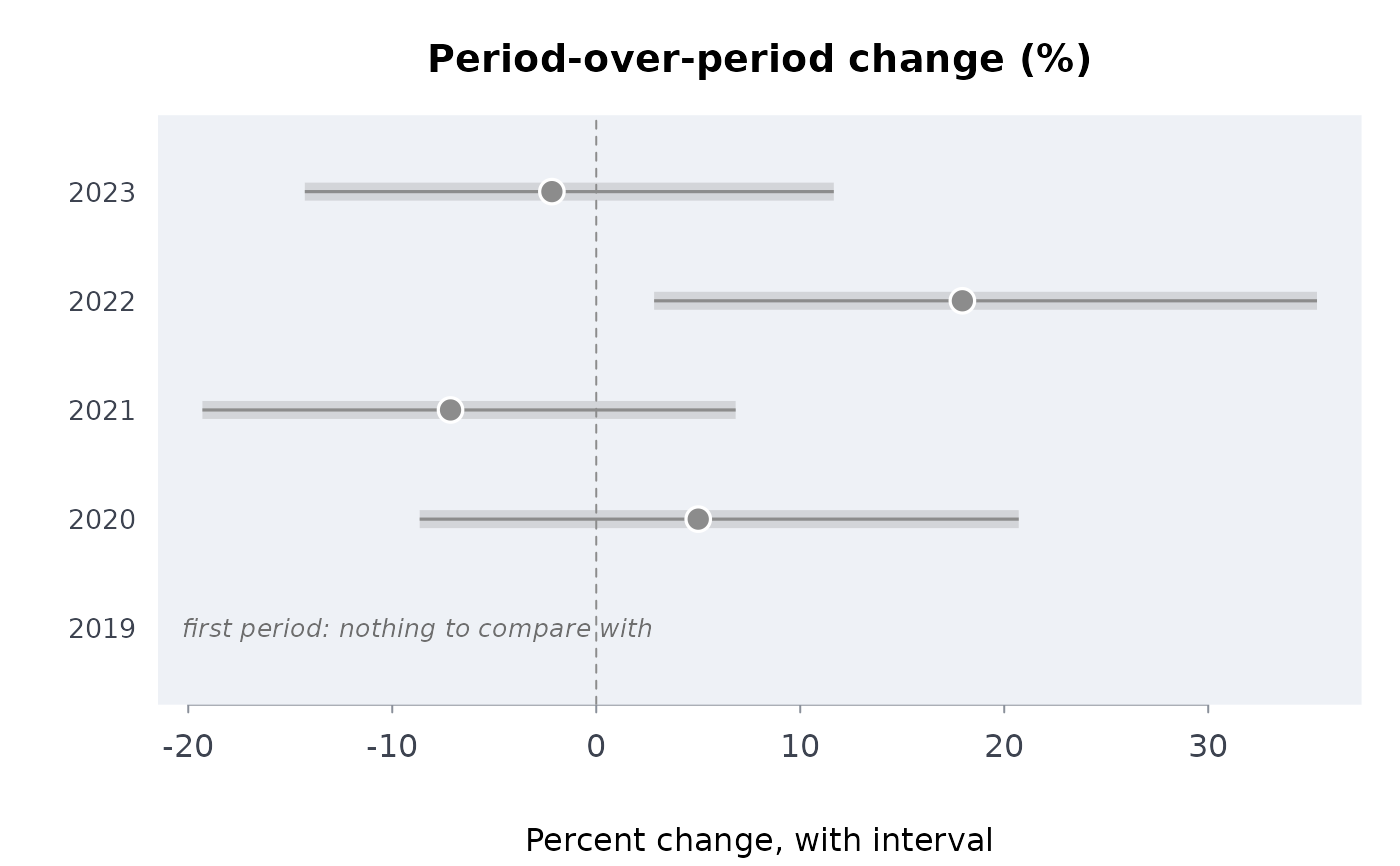
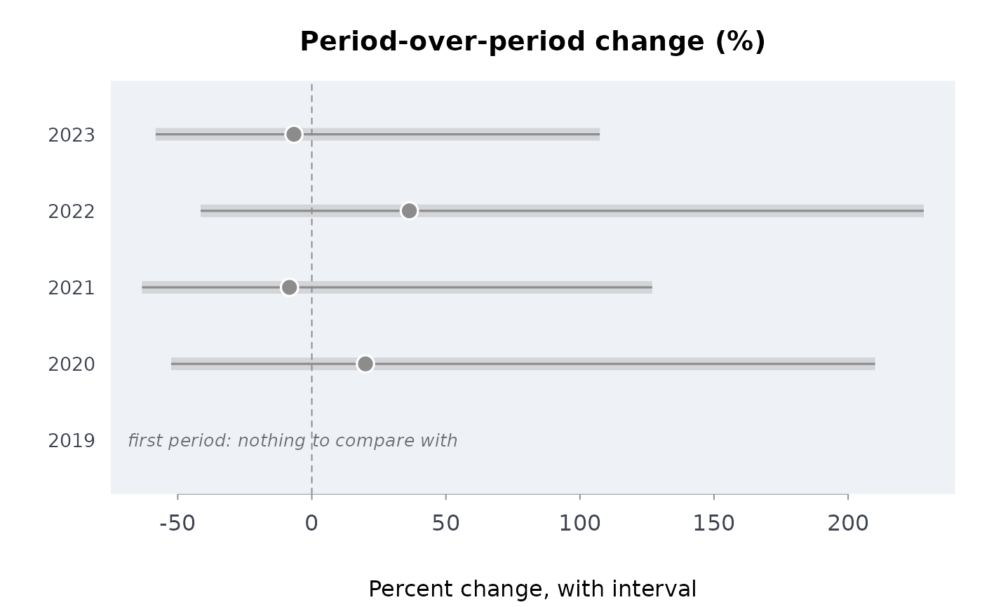
yoy) the period-over-period percent change with its interval, one row per period (and group), coloured by verdict;what = "value"draws the values instead.rmbl_rate,rmbl_share,rmbl_rate_change(
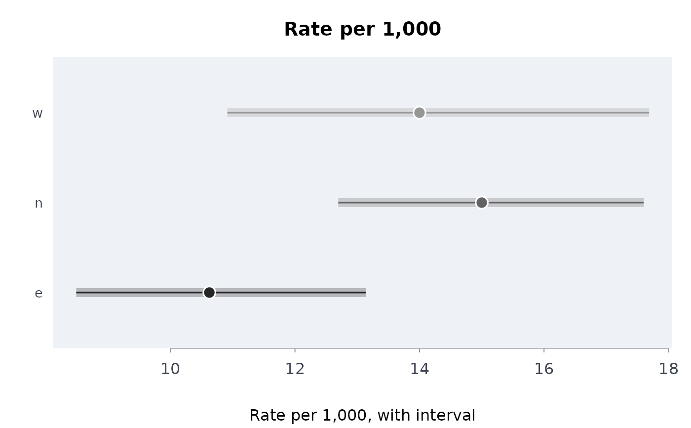
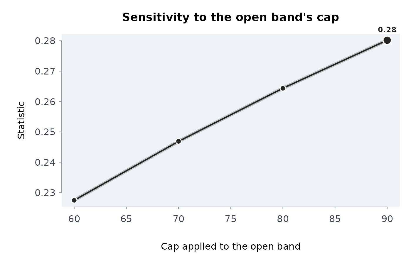
rate) the rate, share or percent change per group with its interval.rmbl_band_sensitivity(
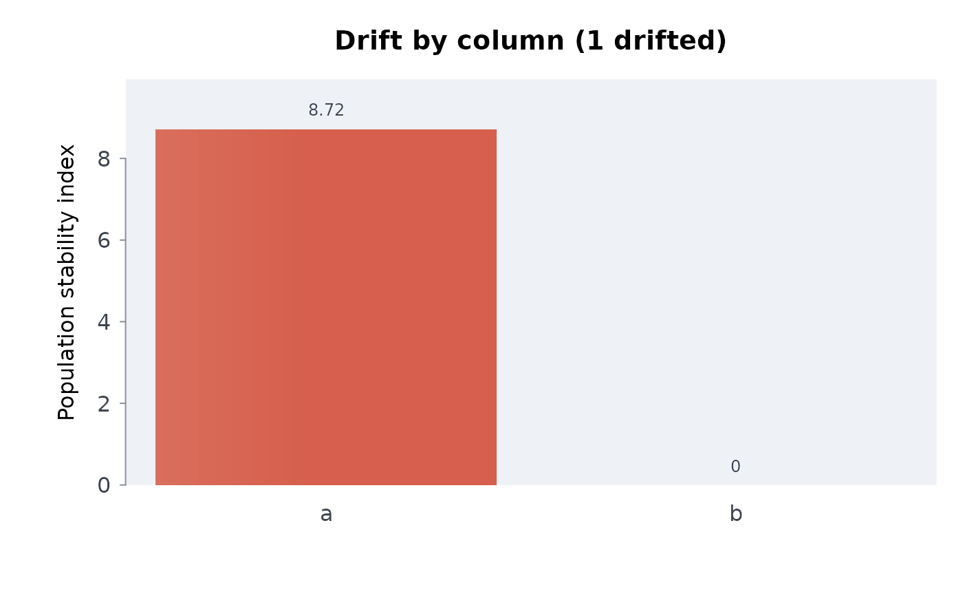
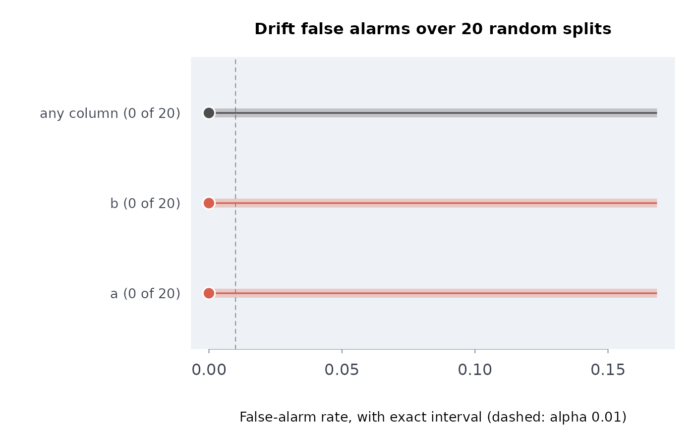
band_sensitivity) the statistic against the cap applied to the open band.rmbl_drift_calibration,bricklayer_drift(
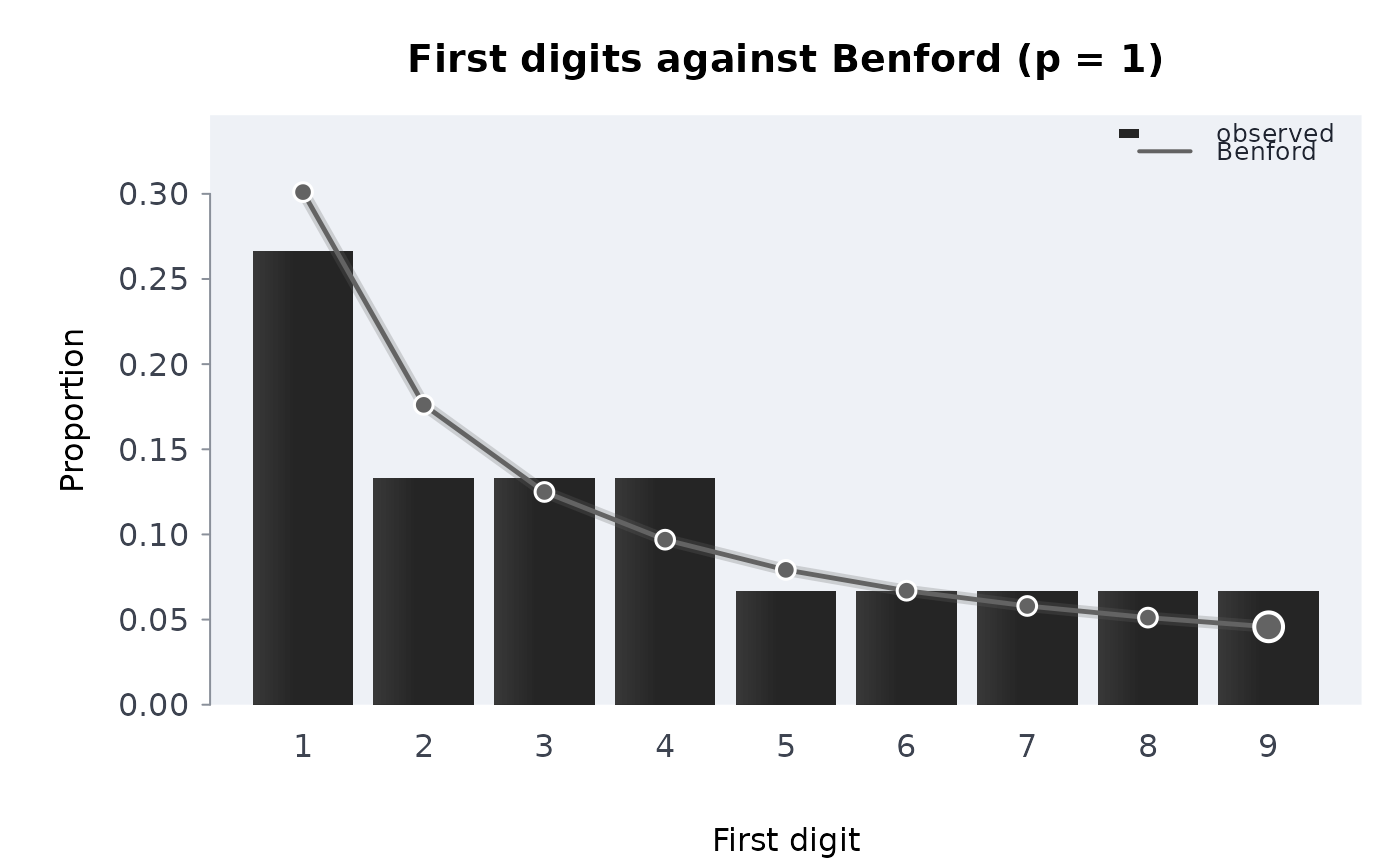
drift_calibrate,capsule_drift) the false-alarm rate per column against alpha; the population stability index per column with the drifted columns marked.bricklayer_benford(
benford_test) observed first-digit proportions against Benford's law.bricklayer_power(
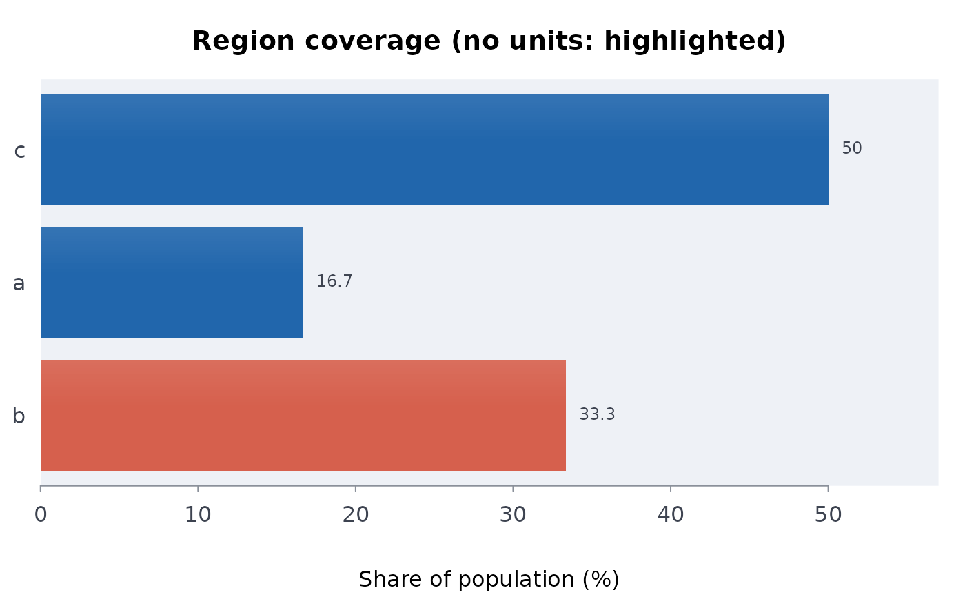
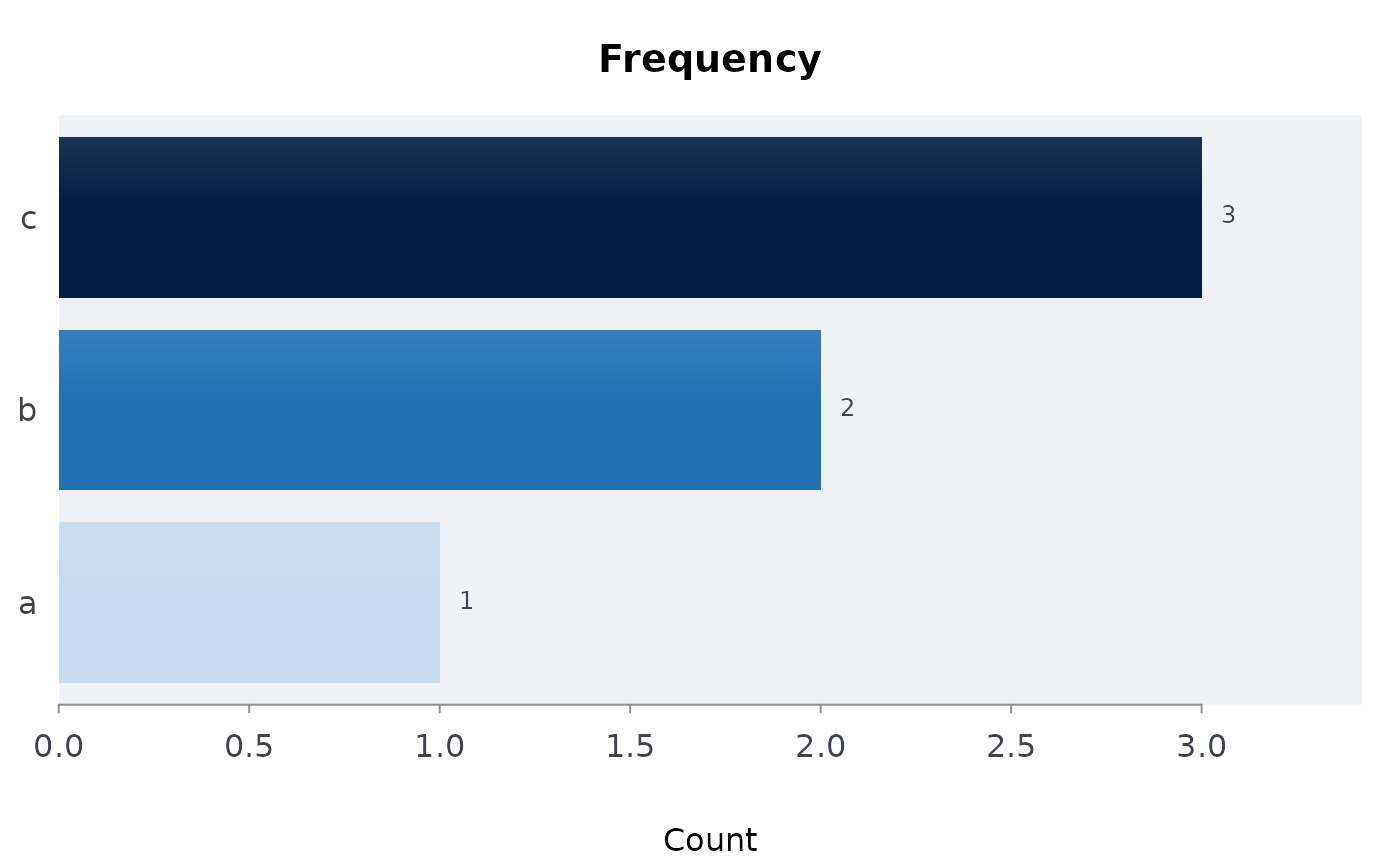
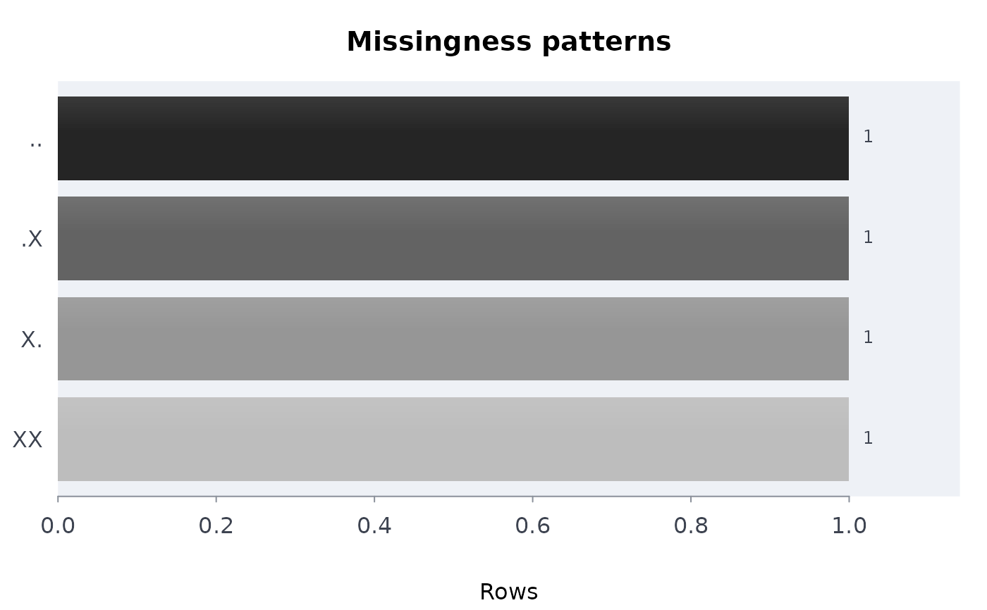
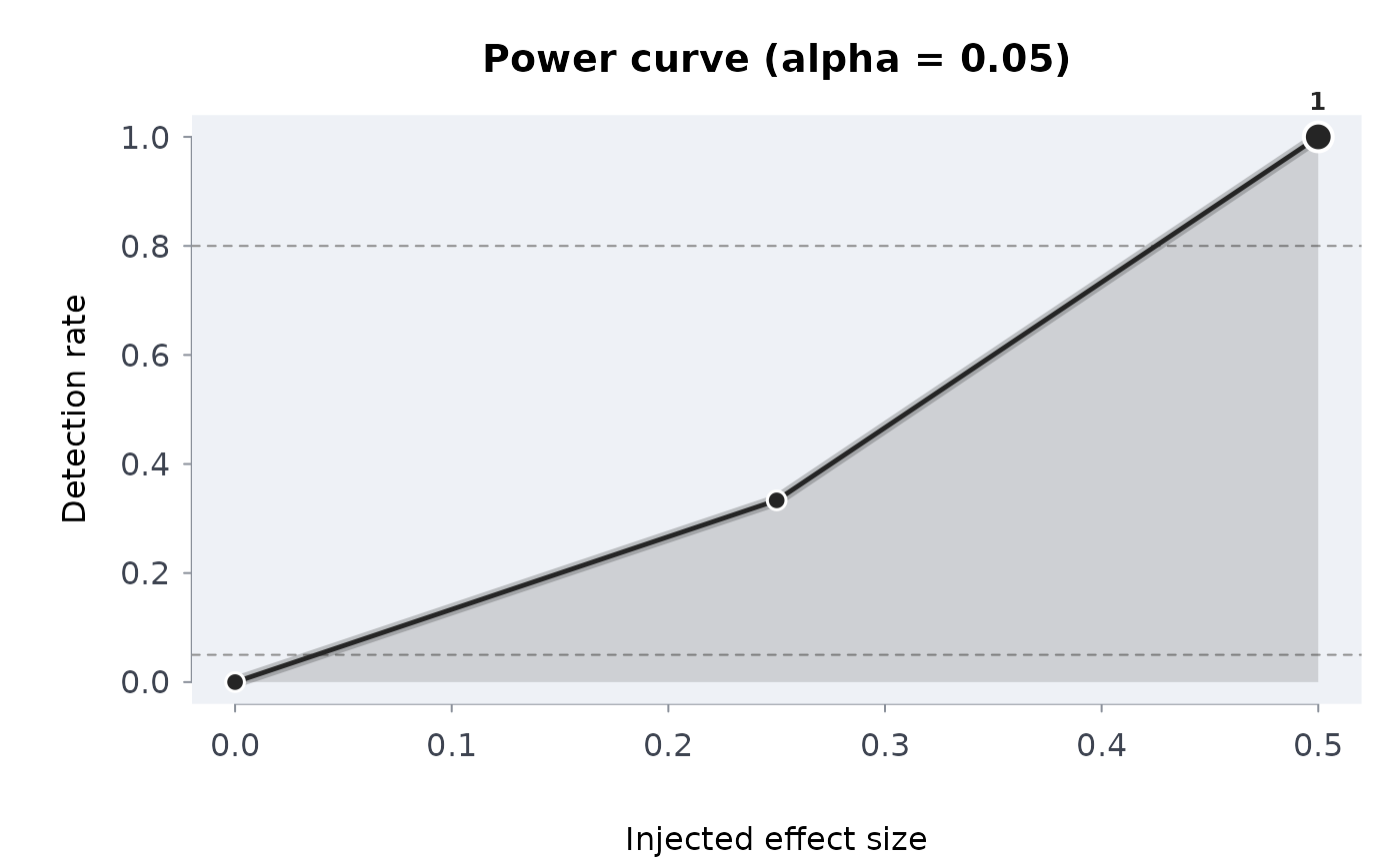
capsule_power) the power curve: detection rate against injected effect size, with the 0.8 line.bricklayer_freq,bricklayer_missingness,rmbl_region_coverage(
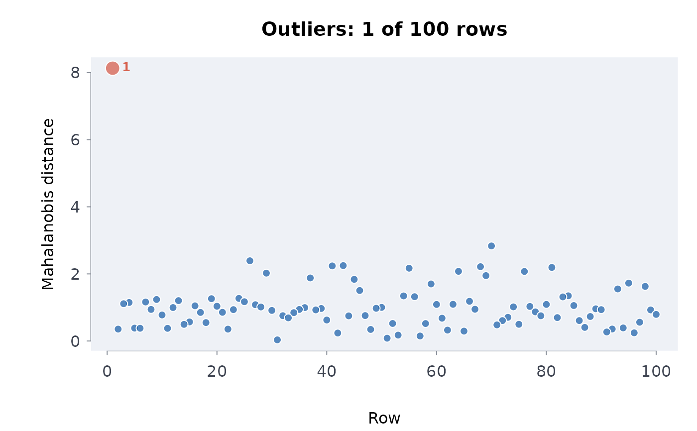
frequency_table,missingness_pattern,region_coverage) horizontal bars.bricklayer_outliers(
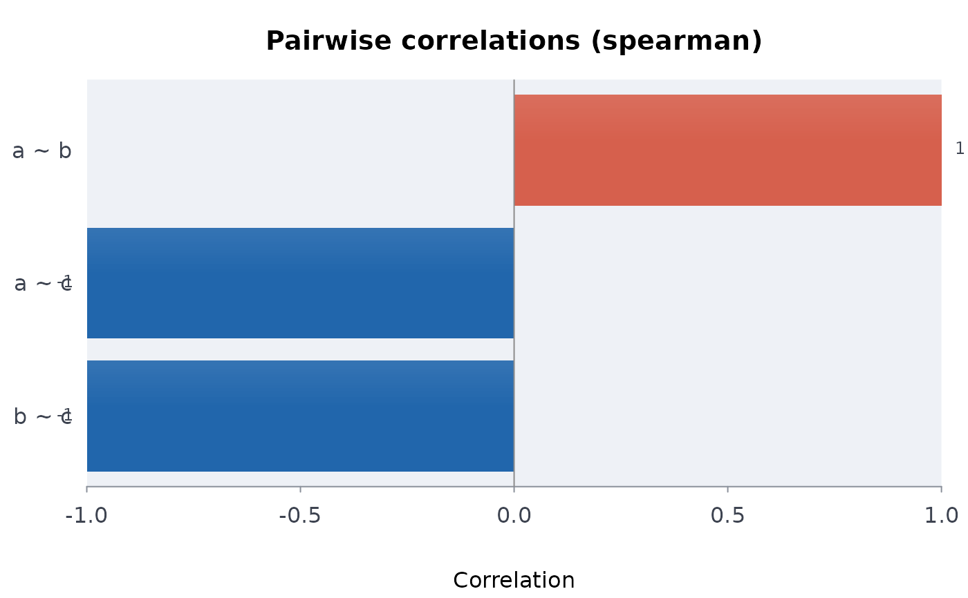
mahalanobis_outliers) the distance of every row, outliers marked.bricklayer_correlations,bricklayer_cortable(
top_correlations,correlation_table) the correlation of every pair as a diverging bar.bricklayer_falsification(
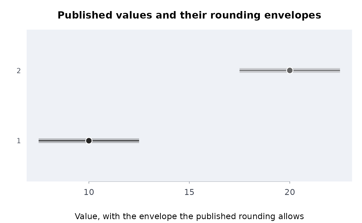
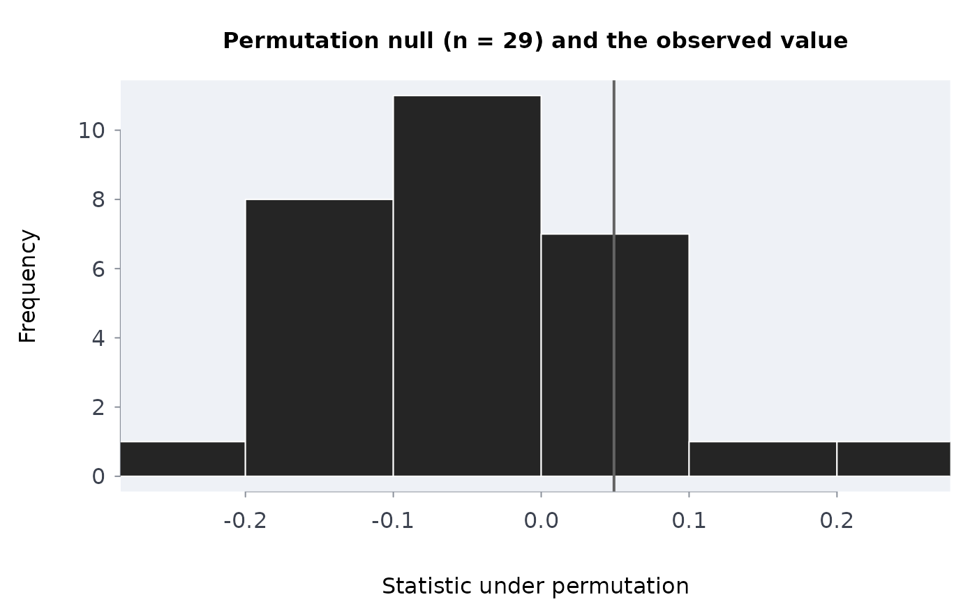
capsule_falsify) the permutation null distribution with the observed statistic.rmbl_bounds(
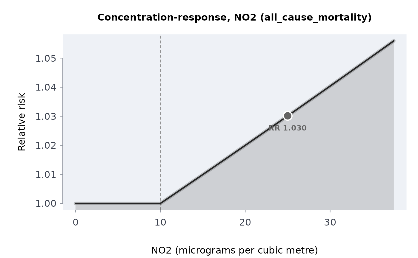
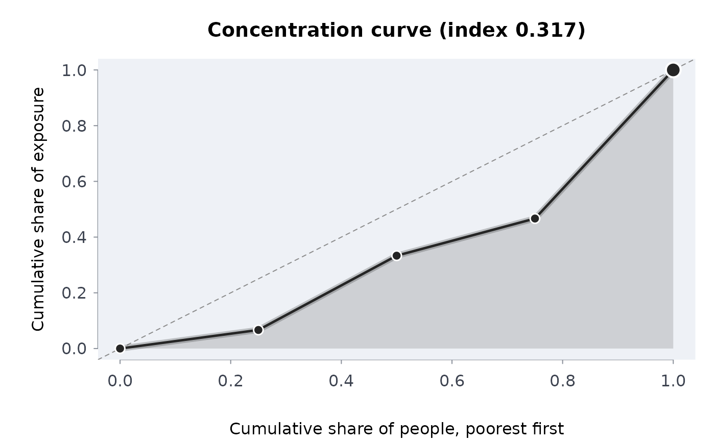
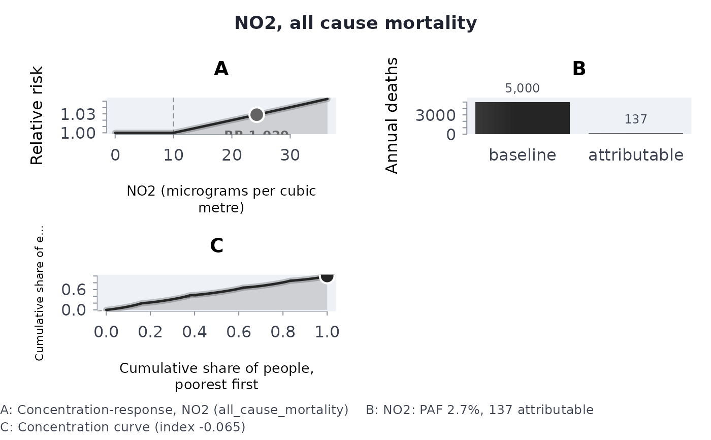
published_bounds) each value inside its published-rounding envelope.rmbl_crf,rmbl_burden,rmbl_equity,rmbl_pollution_report(
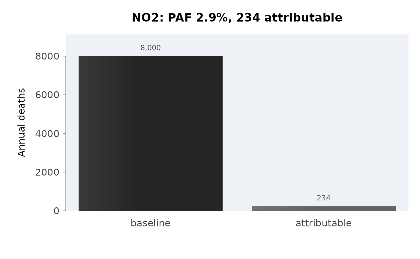
crf_pm25,pollution_burden,exposure_concentration_index,verify_pollution) the concentration-response curve with the exposure marked; baseline against attributable cases; the concentration curve of exposure over income rank; and, for a report, all three on one page.rmbl_footprint(
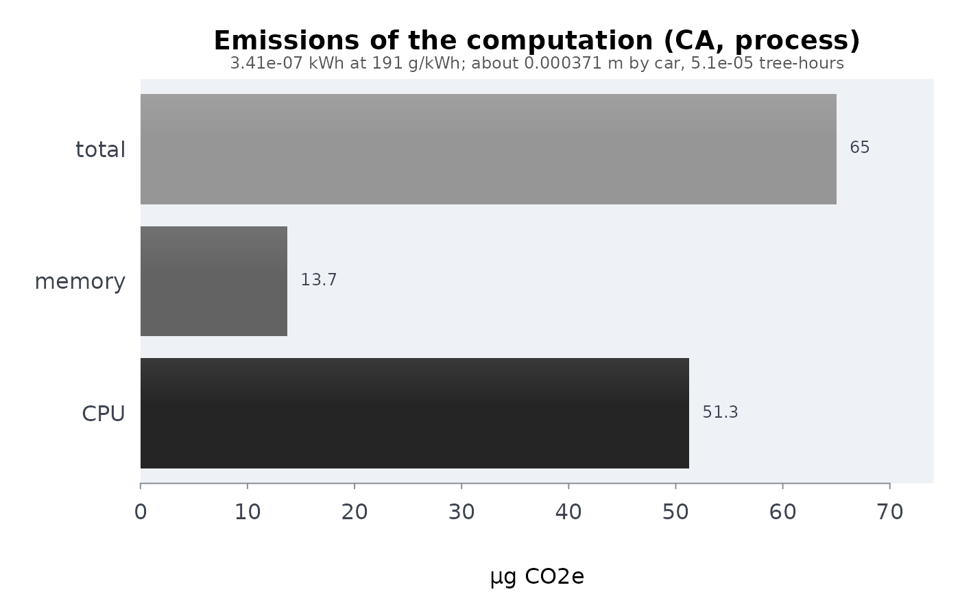
compute_footprint) the CPU, memory and total emission in one unit chosen to fit, with the car-kilometre and tree-month equivalents as a caption; "Too short to measure" when the work took no measurable time.rmbl_field,rmbl_particles(
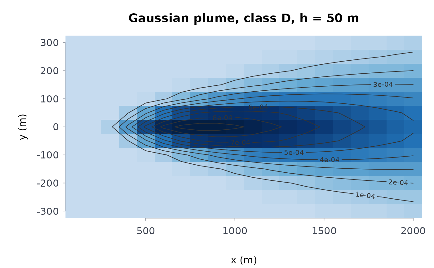
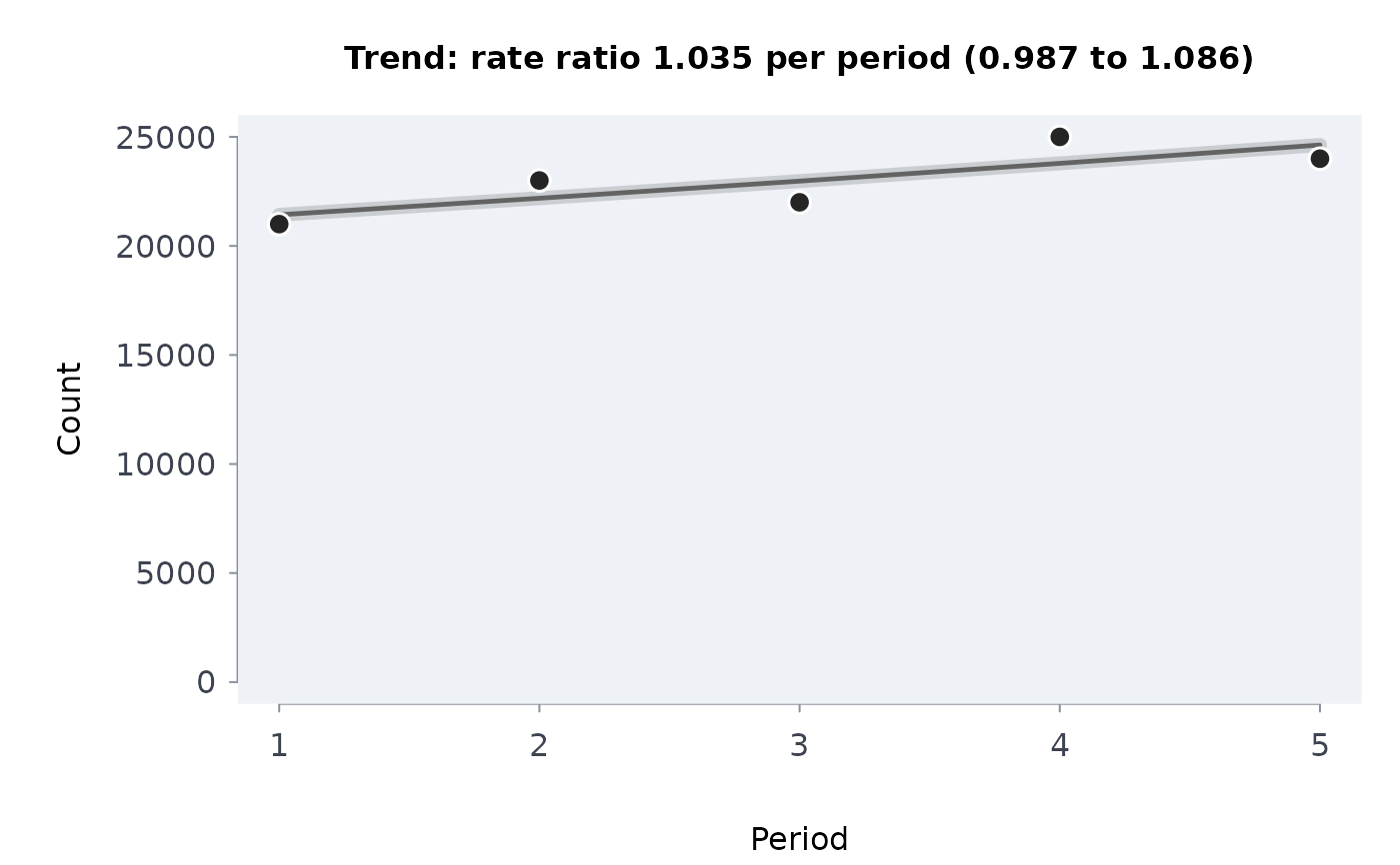
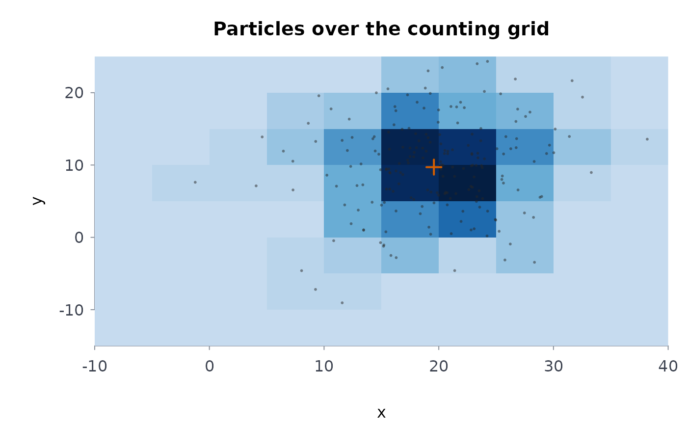
plume_field,advection_diffusion_2d,lagrangian_particles) a concentration field as an image with contours; particle positions, with the counting grid behind them when one was given.rmbl_count_trend(
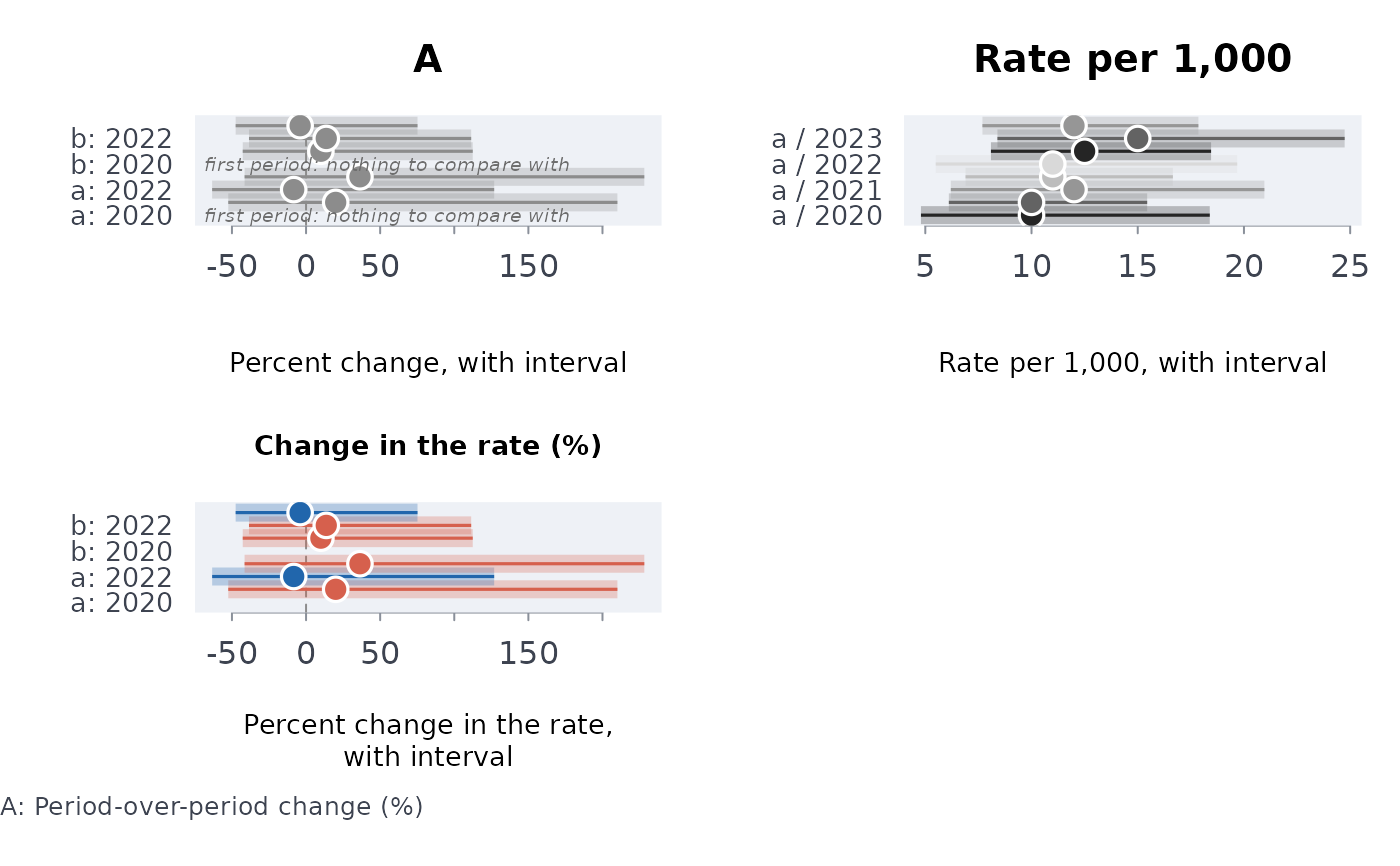
count_trend) the counts with the fitted trend.bricklayer_analysis(
analyse_table) the change, rates and rate change of a published table, one panel each.rmbl_case_flow(
case_flow) cases received and disposed, shaded where the inventory grew or fell, and the clearance rate with its interval and rolling value.rmbl_life_table(
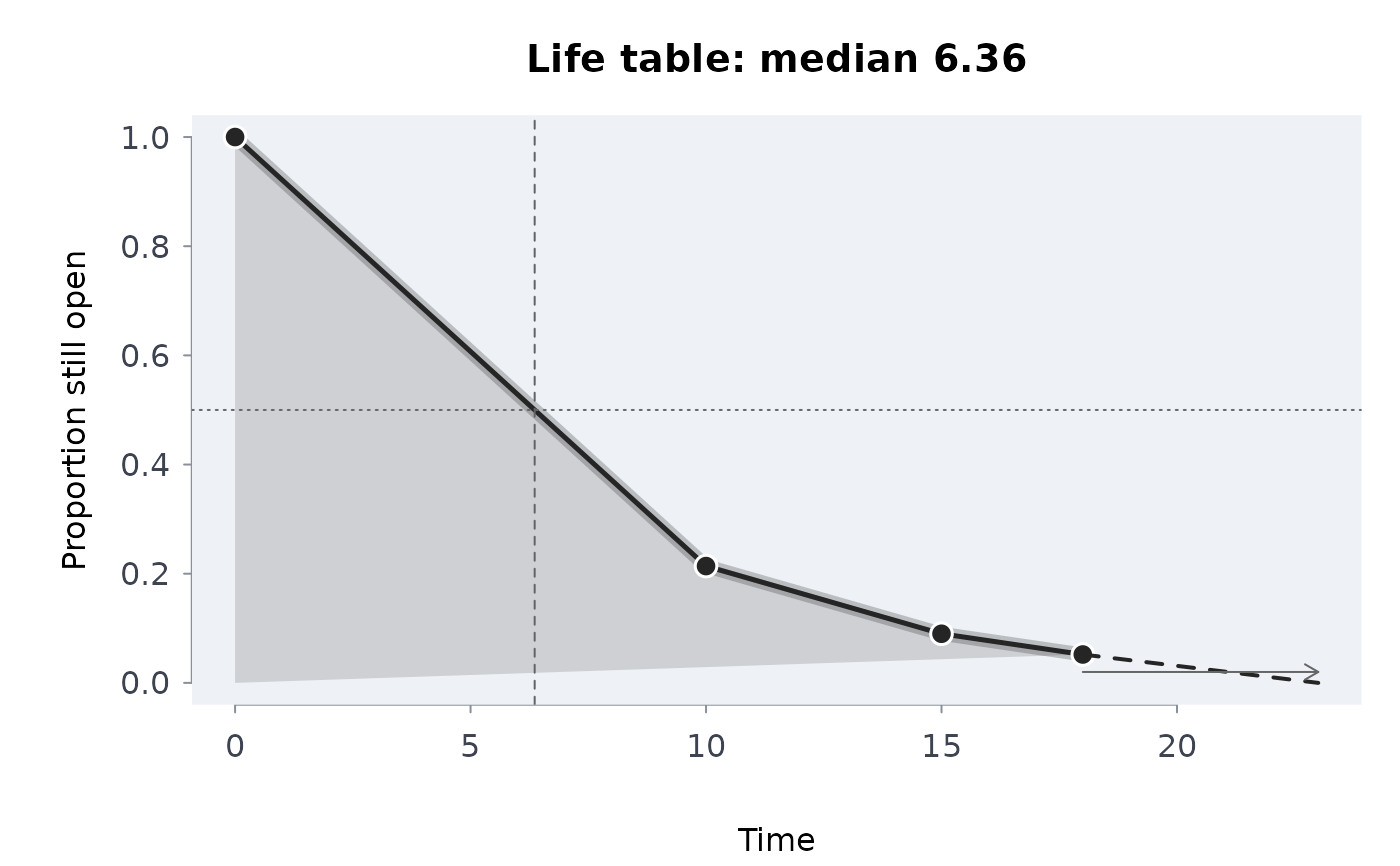
life_table) the share of cases still open at each band edge with its interval, and the median.rmbl_disposition_mix(
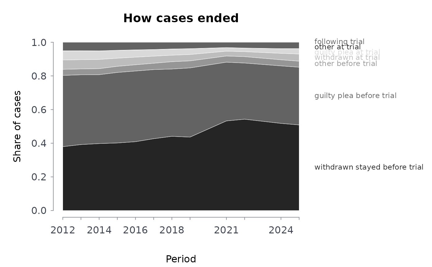
disposition_mix) the shares of each outcome over the periods, stacked.rmbl_density(
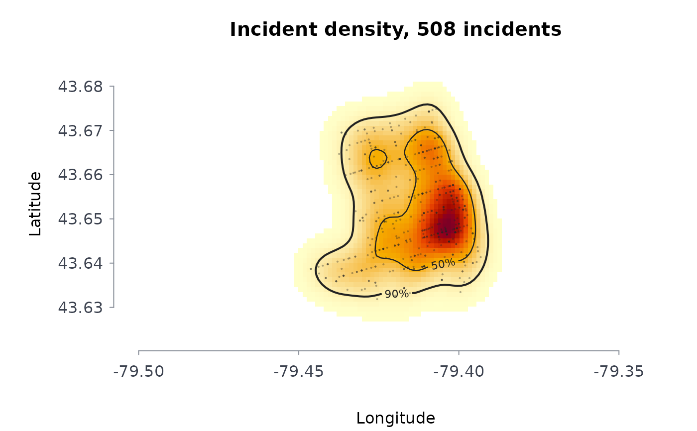
crime_density) the density of incidents as a heat map, with the highest-density regions outlined.rmbl_knox(
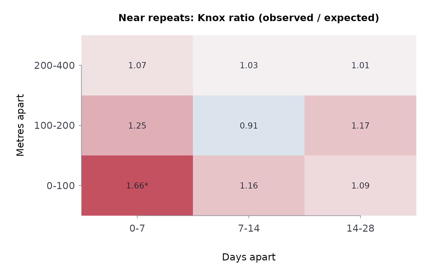
knox_test) the Knox ratio of each distance-by-time cell, coloured on a log scale around 1.rmbl_hotspot(
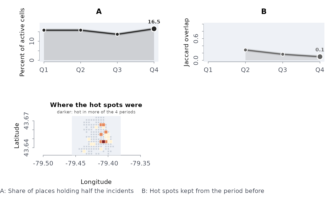
hotspot_persistence) the share of places holding half the incidents and the overlap of hot spots with the period before, over time, and a map of the cells coloured by how often they were hot.rmbl_svy_estimate,rmbl_svy_compare(
survey_estimate,survey_compare) each domain's estimate with its interval, flagged domains marked; each difference from the reference domain with its interval.rmbl_clearance_decomposition(
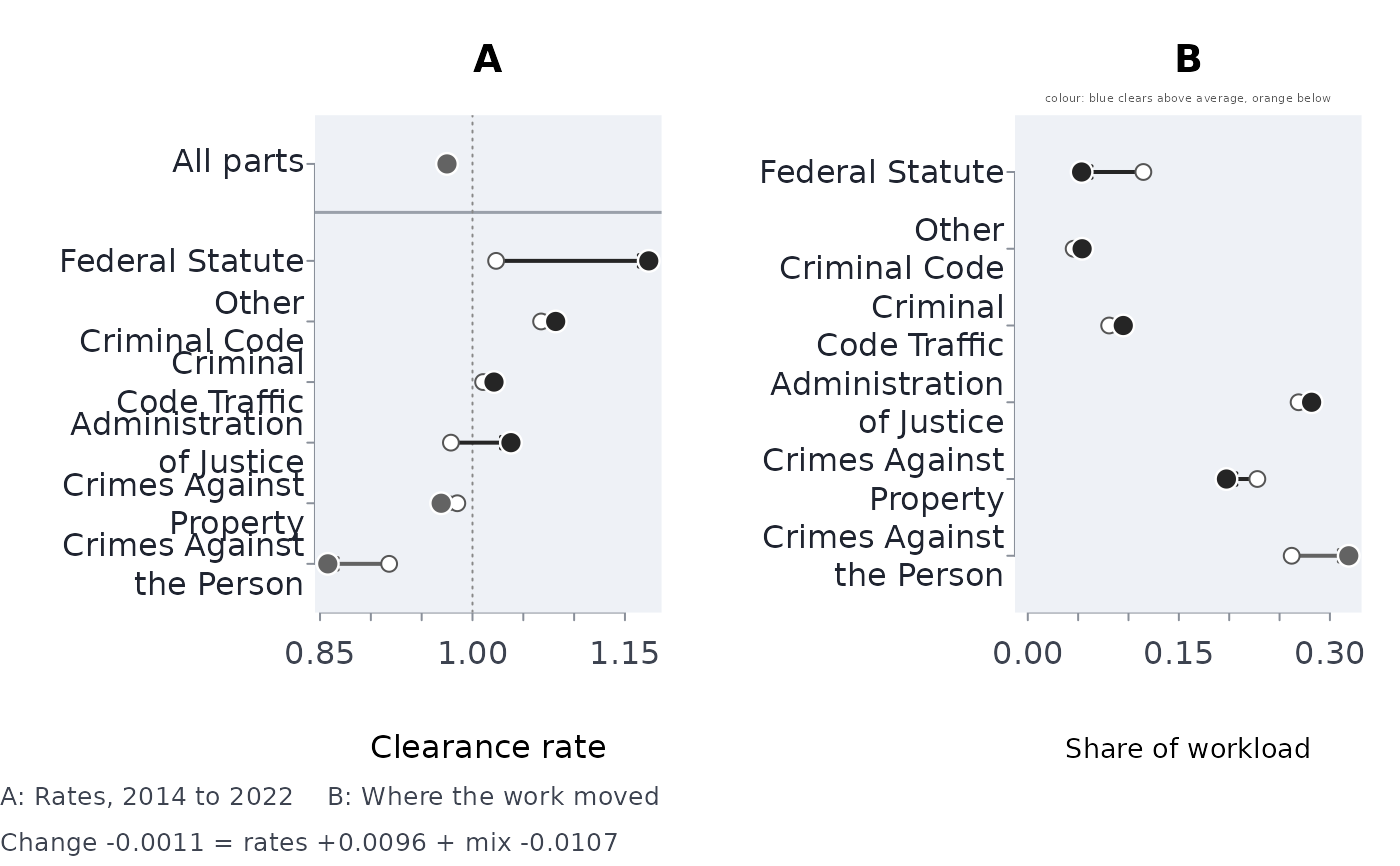
clearance_decomposition) the parts' rates in both comparisons with the aggregate on top, where the workload moved (coloured by whether a part clears above or below the average), and the change as a waterfall of rate and mix effects: the pictures that show a Simpson's-paradox reversal and why it happened.
Examples
sf <- stock_flow(days = c(13500, 14600, 15100), people = c(300, 320, 310),
period = 2021:2023)
plot(sf)
 plot(sf, what = "alos", col = "firebrick", main = "Length of stay")
 y <- yoy(data.frame(year = 2019:2023, n = c(400, 420, 390, 460, 450)), value = "n",
period = "year")
plot(y)
y <- yoy(data.frame(year = 2019:2023, n = c(400, 420, 390, 460, 450)), value = "n",
period = "year")
plot(y)
 # small counts: each percentage carries its exact interval
plot(yoy(data.frame(year = 2019:2023, n = c(10, 12, 11, 15, 14)), value = "n",
period = "year"))
# small counts: each percentage carries its exact interval
plot(yoy(data.frame(year = 2019:2023, n = c(10, 12, 11, 15, 14)), value = "n",
period = "year"))
 plot(benford_test(c(1, 12, 123, 1234, 2, 23, 3, 31, 4, 45, 5, 6, 7, 8, 9)))
 plot(crf_no2(25))
 plot(compute_footprint(for (i in 1:20) sum(sqrt(seq_len(2e5))), location = "CA",
cpu_power_w = 45, memory_gb = 8))
plot(compute_footprint(for (i in 1:20) sum(sqrt(seq_len(2e5))), location = "CA",
cpu_power_w = 45, memory_gb = 8))
 # the courts and crime data shipped with the package
ext <- function(f) {
read.csv(system.file("extdata", f, package = "rmoriebricklayer"))
}
fl <- ext("ocj_flow_ontario.csv")
plot(case_flow(fl$received, fl$disposed, pending = fl$pending, period = fl$month))
# the courts and crime data shipped with the package
ext <- function(f) {
read.csv(system.file("extdata", f, package = "rmoriebricklayer"))
}
fl <- ext("ocj_flow_ontario.csv")
plot(case_flow(fl$received, fl$disposed, pending = fl$pending, period = fl$month))
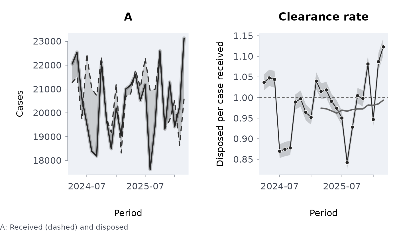 td <- ext("ocj_time_to_disposition.csv")
open <- unlist(td[nrow(td), 2:5]) * fl$disposed[nrow(fl)]
plot(life_table(c(0, 10, 15, 18, Inf), open))
td <- ext("ocj_time_to_disposition.csv")
open <- unlist(td[nrow(td), 2:5]) * fl$disposed[nrow(fl)]
plot(life_table(c(0, 10, 15, 18, Inf), open))
 dm <- ext("ocj_dispositions.csv")
plot(disposition_mix(dm[, -(1:2)], period = dm$year))
dm <- ext("ocj_dispositions.csv")
plot(disposition_mix(dm[, -(1:2)], period = dm$year))
 og <- ext("ocj_offence_groups.csv")
og <- og[og$year %in% c(2014, 2022), ]
plot(clearance_decomposition(og$disposed, og$received, og$offence_group, og$year))
og <- ext("ocj_offence_groups.csv")
og <- og[og$year %in% c(2014, 2022), ]
plot(clearance_decomposition(og$disposed, og$received, og$offence_group, og$year))
 be <- ext("tps_break_enter_d14_2024.csv")
be <- be[!is.na(be$lon), ]
plot(crime_density(be$lon, be$lat, n_grid = 60))
be <- ext("tps_break_enter_d14_2024.csv")
be <- be[!is.na(be$lon), ]
plot(crime_density(be$lon, be$lat, n_grid = 60))
 # \donttest{
plot(knox_test(be$lon, be$lat, as.Date(be$occ_date), c(100, 200, 400), c(7, 14, 28),
nsim = 99, seed = 1))
# \donttest{
plot(knox_test(be$lon, be$lat, as.Date(be$occ_date), c(100, 200, 400), c(7, 14, 28),
nsim = 99, seed = 1))
 # }
plot(hotspot_persistence(be$lon, be$lat, quarters(as.Date(be$occ_date)), cell = 0.3))
# }
plot(hotspot_persistence(be$lon, be$lat, quarters(as.Date(be$occ_date)), cell = 0.3))
 # rates, shares and the change in a rate
rt <- data.frame(division = rep(c("n", "e", "w"), 2), year = rep(2022:2023, each = 3),
stops = c(120, 90, 60, 150, 85, 70),
residents = rep(c(1e4, 8e3, 5e3), 2))
r23 <- rt[rt$year == 2023, ]
plot(rate(r23, count = "stops", population = "residents", by = "division"))
# rates, shares and the change in a rate
rt <- data.frame(division = rep(c("n", "e", "w"), 2), year = rep(2022:2023, each = 3),
stops = c(120, 90, 60, 150, 85, 70),
residents = rep(c(1e4, 8e3, 5e3), 2))
r23 <- rt[rt$year == 2023, ]
plot(rate(r23, count = "stops", population = "residents", by = "division"))
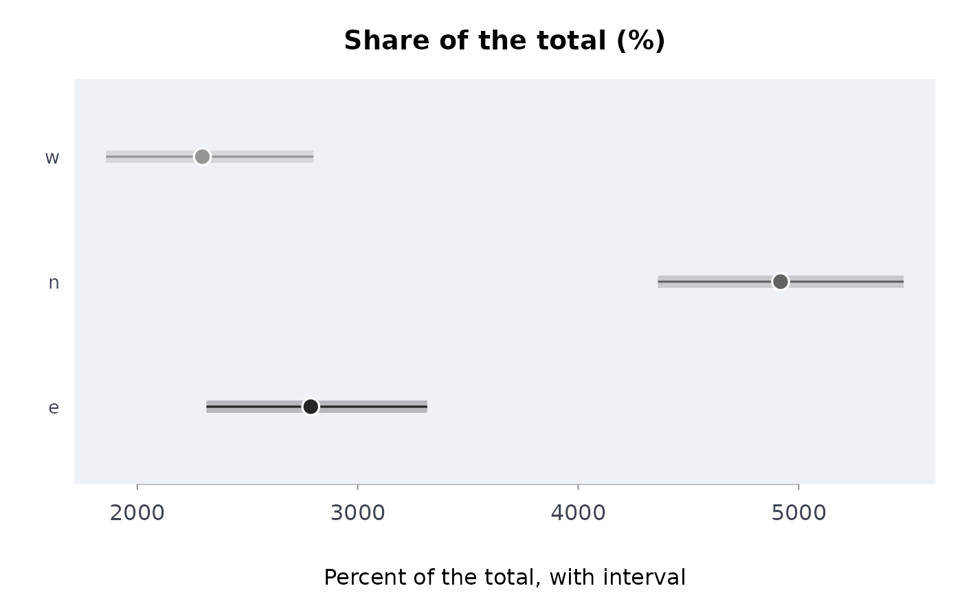
 plot(share(r23, count = "stops", by = "division"))
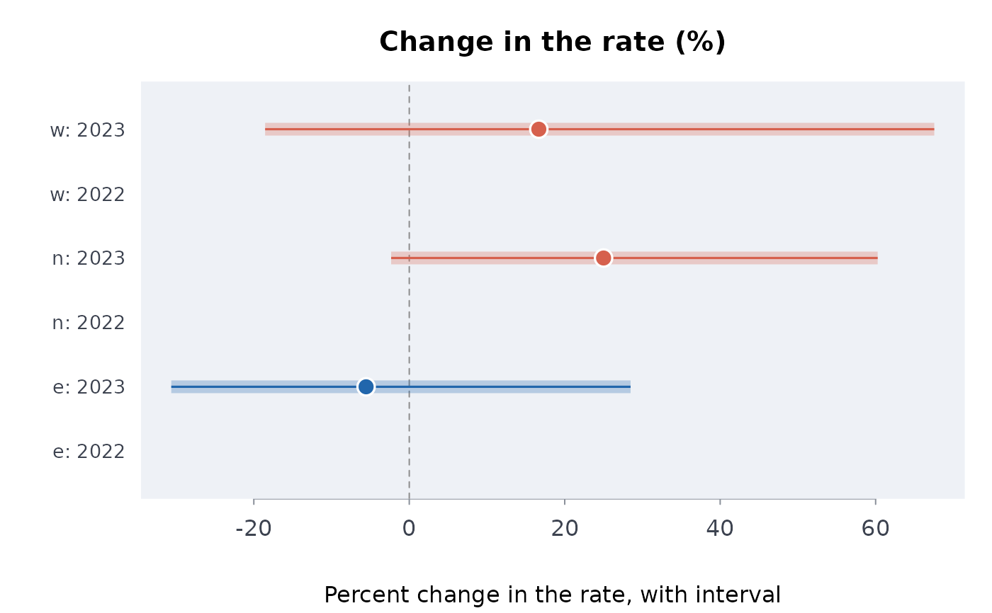
 plot(rate_change(rt, count = "stops", population = "residents", period = "year",
by = "division"))
plot(rate_change(rt, count = "stops", population = "residents", period = "year",
by = "division"))
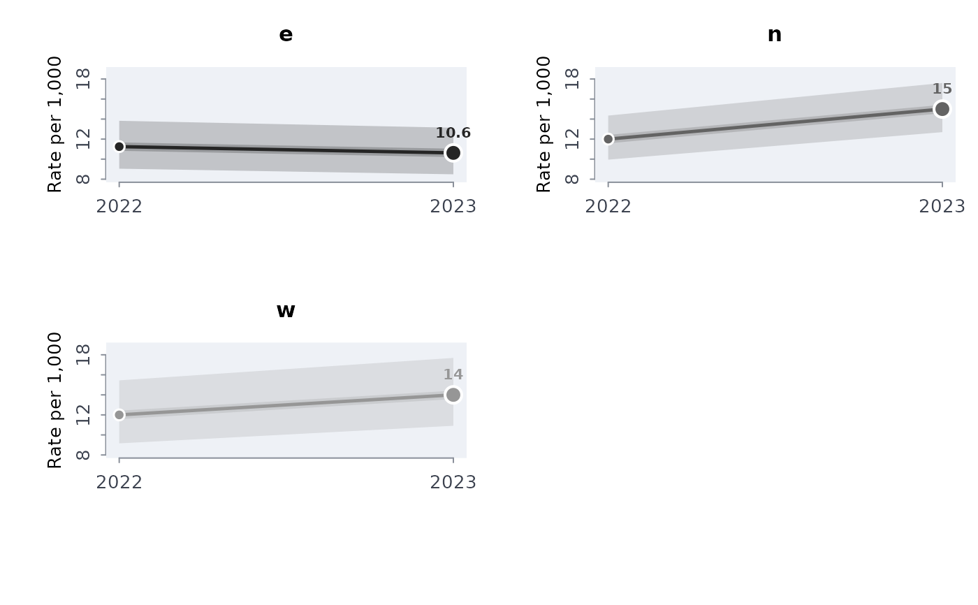
 # a rate over time, one panel per group
plot(rate(rt, count = "stops", population = "residents", by = c("division", "year")),
period = "year")
# a rate over time, one panel per group
plot(rate(rt, count = "stops", population = "residents", by = c("division", "year")),
period = "year")
 # complex survey estimates by domain, and the differences between domains
set.seed(3)
sv <- data.frame(region = rep(c("north", "south", "east"), length.out = 300),
smoker = rbinom(300, 1, 0.25), w = runif(300, 50, 150))
sd <- survey_design(sv, weights = "w", strata = "region")
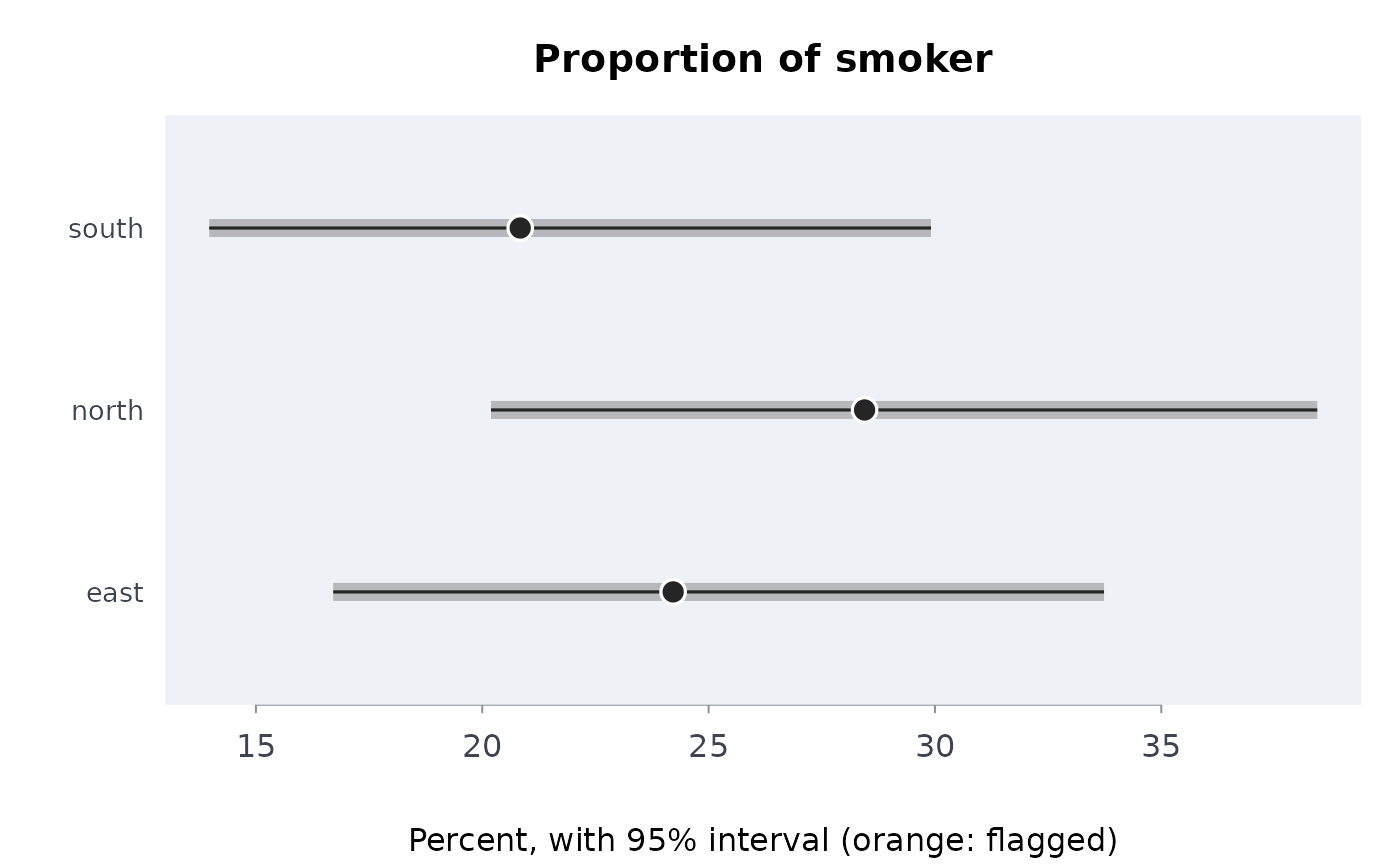
plot(survey_estimate(sd, sv, "smoker", by = "region", stat = "proportion", levels = "1"))
# complex survey estimates by domain, and the differences between domains
set.seed(3)
sv <- data.frame(region = rep(c("north", "south", "east"), length.out = 300),
smoker = rbinom(300, 1, 0.25), w = runif(300, 50, 150))
sd <- survey_design(sv, weights = "w", strata = "region")
plot(survey_estimate(sd, sv, "smoker", by = "region", stat = "proportion", levels = "1"))
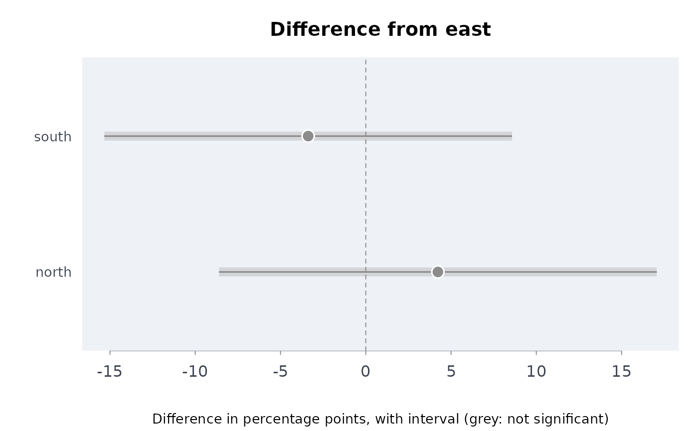
 plot(survey_compare(sd, sv, "smoker", by = "region", stat = "proportion", levels = "1"))
 # a published table in one call: change, rates and rate change
tab <- data.frame(year = rep(2020:2023, each = 2), g = rep(c("a", "b"), 4),
n = c(10, 20, 12, 22, 11, 25, 15, 24), pop = rep(c(1000, 2000), 4))
plot(analyse_table(tab, value = "n", period = "year", by = "g", population = "pop"))
# a published table in one call: change, rates and rate change
tab <- data.frame(year = rep(2020:2023, each = 2), g = rep(c("a", "b"), 4),
n = c(10, 20, 12, 22, 11, 25, 15, 24), pop = rep(c(1000, 2000), 4))
plot(analyse_table(tab, value = "n", period = "year", by = "g", population = "pop"))
 plot(count_trend(c(21000, 23000, 22000, 25000, 24000)))
 # banded tables
plot(band_sensitivity(parse_bands(c("0-17", "18-24", "25-44", "45+")), c(10, 20, 30, 40),
caps = c(60, 70, 80, 90)))
# banded tables
plot(band_sensitivity(parse_bands(c("0-17", "18-24", "25-44", "45+")), c(10, 20, 30, 40),
caps = c(60, 70, 80, 90)))
 plot(published_bounds(c(10, 20), rounding = 5))
 plot(region_coverage(c("a", "b", "c"), c(100, 200, 300), c(1L, 0L, 2L)))
 # drift between two extracts, and how often the test cries wolf
set.seed(1)
dd <- data.frame(a = rnorm(400), b = sample(letters[1:3], 400, TRUE))
plot(capsule_drift(dd, transform(dd, a = a + 3)))
# drift between two extracts, and how often the test cries wolf
set.seed(1)
dd <- data.frame(a = rnorm(400), b = sample(letters[1:3], 400, TRUE))
plot(capsule_drift(dd, transform(dd, a = a + 3)))
 plot(drift_calibrate(dd, n = 20L))
 # describing a table
plot(frequency_table(data.frame(g = c("a", "b", "b", "c", "c", "c")), "g"))
# describing a table
plot(frequency_table(data.frame(g = c("a", "b", "b", "c", "c", "c")), "g"))
 plot(missingness_pattern(data.frame(a = c(1, NA, 3, NA), b = c(NA, NA, 1, 2))))
 hw <- data.frame(h = rnorm(100), w = rnorm(100))
hw$h[1] <- 15
plot(mahalanobis_outliers(hw))
hw <- data.frame(h = rnorm(100), w = rnorm(100))
hw$h[1] <- 15
plot(mahalanobis_outliers(hw))
 sq <- data.frame(a = 1:20, b = (1:20)^2, c = rev(1:20))
plot(top_correlations(sq))
sq <- data.frame(a = 1:20, b = (1:20)^2, c = rev(1:20))
plot(top_correlations(sq))
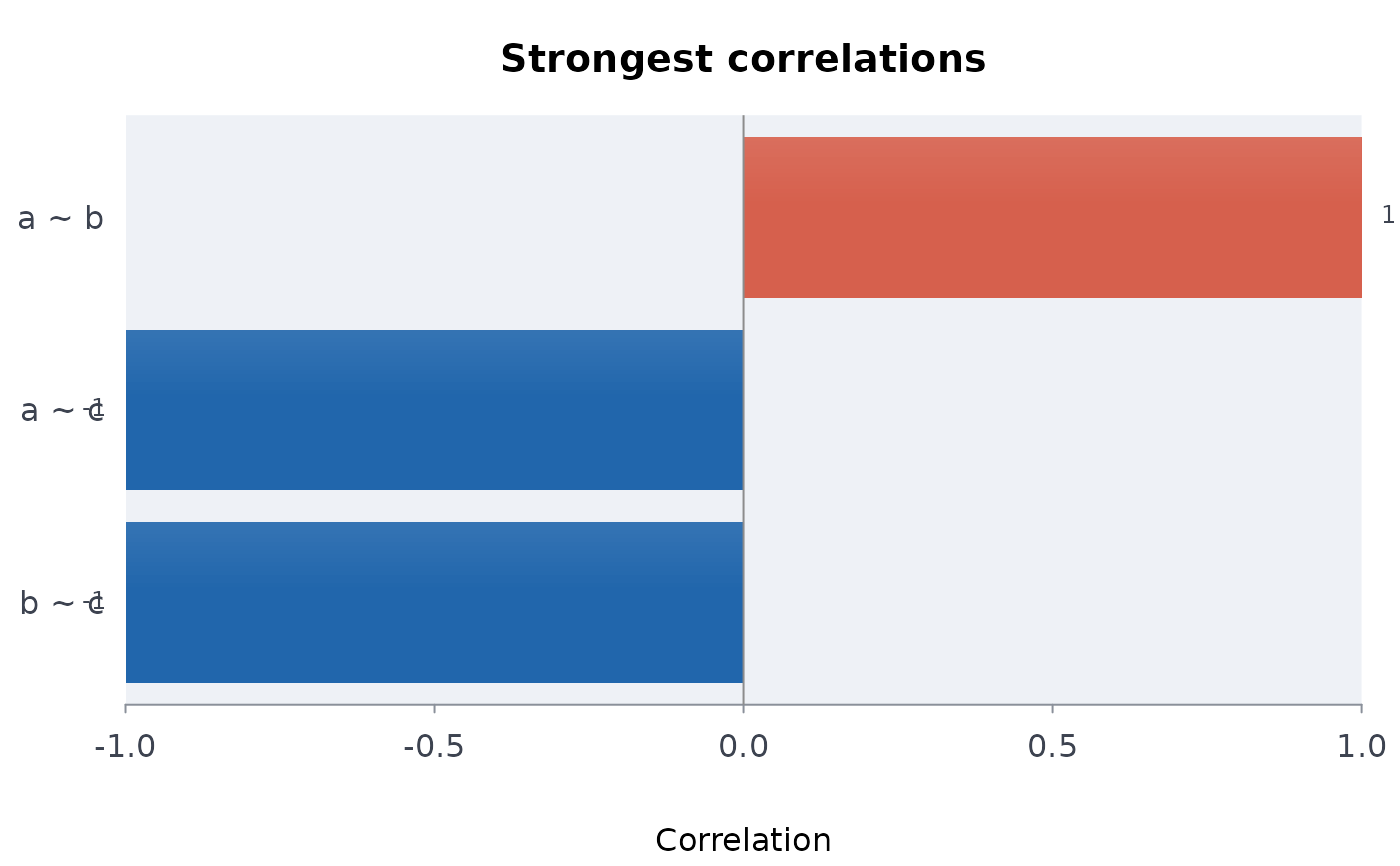 plot(correlation_table(sq))
 # power and falsification of a statistic
xy <- data.frame(x = rnorm(60), y = rnorm(60))
shift <- function(z, s) {
z$y <- z$y + s * z$x
z
}
plot(capsule_power(xy, function(z) cor(z$x, z$y), inject = shift, treatment = "x",
sizes = c(0, 0.25, 0.5), n = 19, reps = 3, seed = 1))
# power and falsification of a statistic
xy <- data.frame(x = rnorm(60), y = rnorm(60))
shift <- function(z, s) {
z$y <- z$y + s * z$x
z
}
plot(capsule_power(xy, function(z) cor(z$x, z$y), inject = shift, treatment = "x",
sizes = c(0, 0.25, 0.5), n = 19, reps = 3, seed = 1))
 plot(capsule_falsify(xy, function(z) cor(z$x, z$y), treatment = "x", n = 29, seed = 1))
 # air pollution: burden, equity, and the full report
plot(pollution_burden(25, 1, 0.008, 1e6, pollutant = "NO2"))
# air pollution: burden, equity, and the full report
plot(pollution_burden(25, 1, 0.008, 1e6, pollutant = "NO2"))
 plot(exposure_concentration_index(data.frame(exposure = c(4, 1, 8, 2),
income = c(2, 1, 4, 3)),
"exposure", "income"))
plot(exposure_concentration_index(data.frame(exposure = c(4, 1, 8, 2),
income = c(2, 1, 4, 3)),
"exposure", "income"))
 plot(verify_pollution("no2", demo = TRUE))
 plot(lagrangian_particles(200, 0, 0, 1, 0.5, 1, 1, 1, 20,
grid = c(-10, 40, -15, 25, 10, 8)))
plot(lagrangian_particles(200, 0, 0, 1, 0.5, 1, 1, 1, 20,
grid = c(-10, 40, -15, 25, 10, 8)))
 plot(plume_field(q = 100, u = 5, h = 50, x = seq(100, 2000, by = 100),
y = seq(-300, 300, by = 50)))
plot(plume_field(q = 100, u = 5, h = 50, x = seq(100, 2000, by = 100),
y = seq(-300, 300, by = 50)))