Life table for grouped times: how long cases take

The actuarial (Cutler-Ederer) life table for times published only in bands – for example the share of court cases disposed within 10 months, between 10 and 15 months, and so on. It gives, at the end of each band, the proportion still open (the survival function) with a Greenwood confidence interval, the hazard within the band, and the median time.

Usage

life_table(
  breaks,
  events,
  censored = 0,
  conf_level = 0.95,
  conf_type = c("log-log", "log", "plain")
)

Arguments

breaks: Band edges, increasing, starting at the time origin: c(0, 10, 15, 18, Inf) for the four bands above. The last edge may be Inf (an open band). Or band labels such as c("Under 10", "10-15", "15-18", "Over 18"), read with parse_bands.
events: Cases that ended in each band (counts, or expected counts such as a published share times the number of cases).
censored: Cases withdrawn from observation in each band without the event (still open when the data were drawn); one value or one per band. Default 0.
conf_level: Confidence level. Default 0.95.
conf_type: Scale of the interval: "log-log" (the default, which keeps the limits inside 0 to 1), "log" or "plain".

Value

A data frame of class rmbl_life_table, one row per band: lower, upper (the band edges), entering, events, censored, at_risk (entering less half the censored), q (conditional probability of the event in the band), survival at the end of the band with se, conf_lower and conf_upper, hazard (events per unit time within the band; NA for an open band), and the attribute median.

Details

Within a band the censored cases are assumed to have been at risk for half of it, so the number at risk is \(n'_j = n_j - c_j/2\); the conditional probability of the event is \(q_j = d_j / n'_j\) and the survival at the end of band \(j\) is \(\prod_{i \le j} (1 - q_i)\). Greenwood's formula gives \(\mathrm{Var}(\hat S_j) = \hat S_j^2 \sum_{i \le j} q_i / (n'_i (1 - q_i))\). With no censoring the table equals the Kaplan-Meier estimate at the band edges, and the Greenwood variance equals the one survival::survfit() reports. The hazard in a closed band is \(d_j / (w_j (n'_j - d_j / 2))\) for band width \(w_j\). The median is interpolated linearly inside the band where survival crosses one half, which assumes events are spread evenly across that band; when the crossing falls in an open band, the median is reported as greater than its lower edge.

Court statistics that count only disposed cases describe time to disposition among cases that were disposed, with no censoring; cases still pending are not in them, so the survival function describes the disposed cohort, not every case received.

The median is attribute "median" (Inf, with a note, when survival never falls to one half or crosses it in the open band), and attribute "life_table" records conf_level and conf_type. Errors: band labels that cannot be read, or that are not contiguous, or with an open band other than the last; fewer than two increasing edges, or an infinite edge other than the last; events or censored that are not non-negative counts, one per band; no cases at all; conf_level outside (0, 1); an unknown conf_type.

References

Cutler, S. J. and Ederer, F. (1958). Maximum utilization of the life table method in analyzing survival. Journal of Chronic Diseases, 8(6), 699-712.

Greenwood, M. (1926). The Natural Duration of Cancer. Reports on Public Health and Medical Subjects 33. HMSO, London.

Lee, E. T. and Wang, J. W. (2003). Statistical Methods for Survival Data Analysis, 3rd ed. Wiley, Hoboken, NJ. Chapter 4.

Examples

d <- read.csv(system.file("extdata", "ocj_time_to_disposition.csv",
                          package = "rmoriebricklayer"))
f <- read.csv(system.file("extdata", "ocj_flow_ontario.csv",
                          package = "rmoriebricklayer"))
last <- nrow(d)
shares <- unlist(d[last, c("under_10", "m10_15", "m15_18", "over_18")])
lt <- life_table(c(0, 10, 15, 18, Inf), events = shares * f$disposed[last])
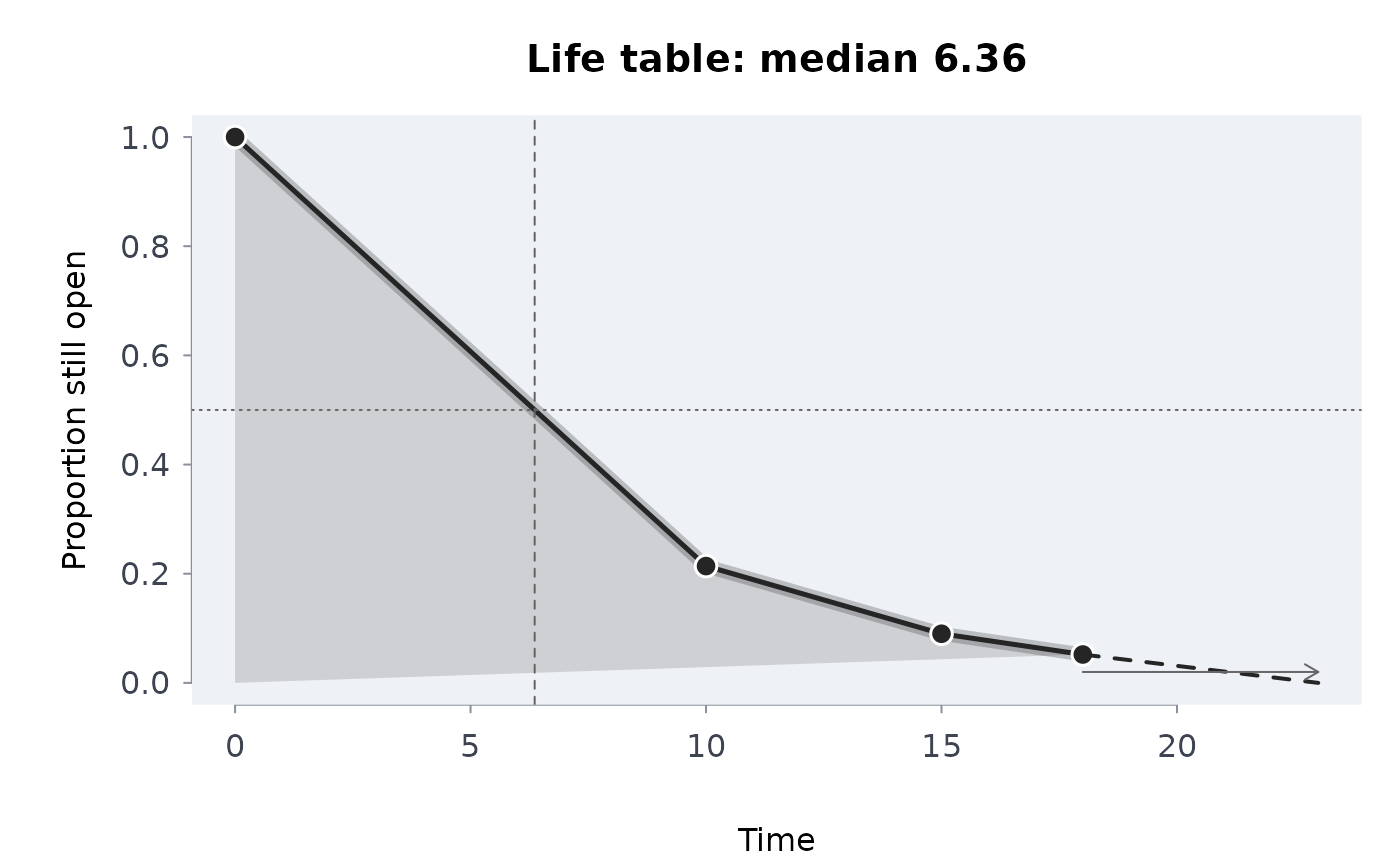
lt
#> ── Life table (actuarial), 95% log-log Greenwood interval ──────── 
#>   Median time: 6.36 (linear within its band)
#> 
#>  lower upper  entering    events censored   at_risk      q survival     se
#>      0    10 23136.000 18184.896        0 23136.000 0.7860    0.214 0.0027
#>     10    15  4951.104  2868.864        0  4951.104 0.5794    0.090 0.0019
#>     15    18  2082.240   879.168        0  2082.240 0.4222    0.052 0.0015
#>     18   Inf  1203.072  1203.072        0  1203.072 1.0000    0.000     NA
#>  conf_lower conf_upper hazard
#>      0.2087     0.2193 0.1295
#>      0.0864     0.0937 0.1632
#>      0.0492     0.0549 0.1784
#>          NA         NA     NA
#> ────────────────────────────────────────────────────────────────── 
plot(lt)


# bands given by their labels, with some cases still open, on the log scale
lt2 <- life_table(c("Under 10", "10-15", "15-18", "Over 18"),
                  events = c(600, 150, 60, 90), censored = c(40, 20, 10, 0),
                  conf_type = "log")
as.data.frame(lt2)[, c("lower", "upper", "at_risk", "survival",
                       "conf_lower", "conf_upper")]
#>   lower upper at_risk  survival conf_lower conf_upper
#> 1     0    10     950 0.3684211 0.33898914  0.4004083
#> 2    10    15     320 0.1957237 0.17145569  0.2234266
#> 3    15    18     155 0.1199597 0.09998399  0.1439263
#> 4    18   Inf      90 0.0000000         NA         NA
attr(lt2, "median")
#> [1] 7.916667

# an open band can only come last
try(life_table(c(0, Inf, 20), events = c(5, 5)))
#> Error : `breaks` must be at least two increasing band edges