
Turns the counts a court publishes each period – cases received, cases disposed and, when it is published, cases pending – into the measures used to judge whether a court is keeping up: the clearance rate (cases disposed per case received), its rolling value over a window, the net flow into the inventory and, with the pending count, the number of periods the current inventory would take to clear at the recent pace of disposition.
Usage
case_flow(
  received,
  disposed,
  pending = NULL,
  period = NULL,
  window = 12L,
  conf_level = 0.95
)
Arguments
- received
Cases received (new cases), one per period, in time order.
- disposed
Cases disposed, one per period.
- pending
Optional cases pending at the end of each period.
- period
Optional period labels: numbers, dates, or
"YYYY-MM"strings (which the plot draws on a date axis).- window
Periods in the rolling clearance rate and in the pace behind
periods_to_clear. Default 12, a year of months.- conf_level
Confidence level for the intervals. Default 0.95.
Value
A data frame of class rmbl_case_flow, one row per period:
period, received, disposed, clearance with
lower and upper, net (received less disposed:
positive grows the inventory), rolling_clearance with
rolling_lower and rolling_upper (NA until a full
window is available), and either pending,
pending_change and periods_to_clear, or, without
pending, cumulative_net (the inventory change since the
first period).
Details
A clearance rate above 1 means the court disposed of more cases than it received, so its inventory fell. The interval treats received and disposed as Poisson counts over the same period: given their sum, the disposed count is binomial, and the exact (Clopper-Pearson) limits for that proportion give exact limits for the ratio. The interval measures the period-to-period noise of counts this size; it does not make received and disposed the same cases, which they are not (a case disposed this month was usually received months before).
periods_to_clear divides the pending inventory by the mean
number disposed over the last window periods (fewer at the start
of the series). The published pending count need not equal the previous
count plus the net flow – courts reactivate cases on bench warrants and
transfer them – so pending_change is reported next to
net rather than derived from it.
The result carries attribute "case_flow": window,
conf_level and the totals received and disposed. Errors:
received empty; a count vector that is not numeric, has a missing,
negative or infinite value, or a length other than received's;
period of another length, with missing or repeated values;
window not a whole number of at least 1; conf_level
outside (0, 1).
References
Ostrom, B. J. and Hanson, R. A. (1999). Efficiency, Timeliness, and Quality: A New Perspective from Nine State Criminal Trial Courts. National Center for State Courts, Williamsburg, VA. (Clearance rate and time-to-disposition measures.)
Ulm, K. (1990). A simple method to calculate the confidence interval of a standardized mortality ratio. American Journal of Epidemiology, 131(2), 373-375. (Exact limits for a ratio of Poisson counts through the beta distribution.)
See also
life_table, disposition_mix,
stock_flow for custody populations.
Examples
f <- read.csv(system.file("extdata", "ocj_flow_ontario.csv",
package = "rmoriebricklayer"))
cf <- case_flow(f$received, f$disposed, pending = f$pending, period = f$month)
cf
#> ── Case flow, 95% exact intervals, 12-period rolling window ──────
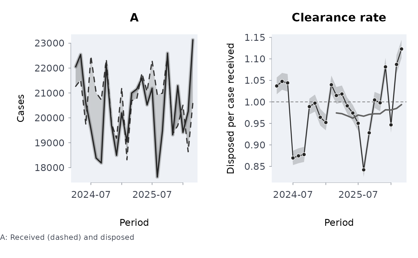
#> Over all 24 periods: 497,393 received, 489,448 disposed, clearance 0.984 (0.980 to 0.988)
#> Pending at the end: 148,473, about 7.2 periods of disposition at the last 12-period pace
#>
#> period received disposed clearance lower upper net rolling_clearance
#> 2024-04 21265 22053 1.037 1.018 1.057 -788 NA
#> 2024-05 21521 22546 1.048 1.028 1.067 -1025 NA
#> 2024-06 19728 20599 1.044 1.024 1.065 -871 NA
#> 2024-07 22483 19552 0.870 0.853 0.887 2931 NA
#> 2024-08 21019 18383 0.875 0.857 0.892 2636 NA
#> 2024-09 20720 18186 0.878 0.860 0.895 2534 NA
#> 2024-10 22349 22104 0.989 0.971 1.008 245 NA
#> 2024-11 19769 19711 0.997 0.978 1.017 58 NA
#> 2024-12 19179 18492 0.964 0.945 0.984 687 NA
#> 2025-01 21210 20196 0.952 0.934 0.971 1014 NA
#> 2025-02 18314 19044 1.040 1.019 1.061 -730 NA
#> 2025-03 20688 20996 1.015 0.996 1.035 -308 0.974
#> 2025-04 20778 21159 1.018 0.999 1.038 -381 0.973
#> 2025-05 21795 21596 0.991 0.972 1.010 199 0.968
#> 2025-06 21064 20519 0.974 0.956 0.993 545 0.962
#> 2025-07 22298 21188 0.950 0.932 0.968 1110 0.969
#> 2025-08 20927 17623 0.842 0.825 0.859 3304 0.967
#> 2025-09 20993 19483 0.928 0.910 0.946 1510 0.971
#> 2025-10 22497 22598 1.004 0.986 1.023 -101 0.972
#> 2025-11 19360 19319 0.998 0.978 1.018 41 0.972
#> 2025-12 19688 21291 1.081 1.061 1.103 -1603 0.982
#> 2026-01 20508 19413 0.947 0.928 0.965 1095 0.981
#> 2026-02 18638 20261 1.087 1.066 1.109 -1623 0.985
#> 2026-03 20602 23136 1.123 1.102 1.144 -2534 0.994
#> pending periods_to_clear
#> 148904 6.8
#> 147957 6.6
#> 145989 6.7
#> 147277 7.0
#> 149417 7.2
#> 151588 7.5
#> 150716 7.4
#> 150270 7.4
#> 151092 7.5
#> 151494 7.5
#> 150772 7.5
#> 150480 7.5
#> 151254 7.5
#> 151239 7.6
#> 149703 7.5
#> 150980 7.5
#> 153629 7.7
#> 153998 7.6
#> 154255 7.6
#> 152825 7.6
#> 151693 7.4
#> 150987 7.4
#> 149760 7.3
#> 148473 7.2
#> ──────────────────────────────────────────────────────────────────
plot(cf)
 # without the pending count, a quarterly rolling window and 90% intervals
cq <- case_flow(f$received, f$disposed, period = f$month, window = 3, conf_level = 0.90)
head(as.data.frame(cq)[, c("period", "clearance", "rolling_clearance", "cumulative_net")])
#> period clearance rolling_clearance cumulative_net
#> 1 2024-04 1.0370562 NA -788
#> 2 2024-05 1.0476279 NA -1813
#> 3 2024-06 1.0441504 1.0429344 -2684
#> 4 2024-07 0.8696348 0.9837601 247
#> 5 2024-08 0.8745897 0.9257315 2883
#> 6 2024-09 0.8777027 0.8738594 5417
# one value per period in every count
try(case_flow(c(100, 120, 90), c(95, 130)))
#> Error : `disposed` must have 3 values (one per period), got 2
# without the pending count, a quarterly rolling window and 90% intervals
cq <- case_flow(f$received, f$disposed, period = f$month, window = 3, conf_level = 0.90)
head(as.data.frame(cq)[, c("period", "clearance", "rolling_clearance", "cumulative_net")])
#> period clearance rolling_clearance cumulative_net
#> 1 2024-04 1.0370562 NA -788
#> 2 2024-05 1.0476279 NA -1813
#> 3 2024-06 1.0441504 1.0429344 -2684
#> 4 2024-07 0.8696348 0.9837601 247
#> 5 2024-08 0.8745897 0.9257315 2883
#> 6 2024-09 0.8777027 0.8738594 5417
# one value per period in every count
try(case_flow(c(100, 120, 90), c(95, 130)))
#> Error : `disposed` must have 3 values (one per period), got 2