
The mix of outcomes over time, with simultaneous intervals and trend tests
Source:R/justice.R
disposition_mix.RdFor a table of counts – periods in rows, outcomes in columns, such as cases withdrawn, pleaded guilty, or tried – gives each outcome's share of its period with Goodman's simultaneous confidence intervals, tests whether the mix is the same in every period, and tests each outcome for a linear trend in its share.
Arguments
- counts
A matrix or data frame of non-negative counts, one row per period and one column per outcome. Columns that are not numeric are refused; pass only the outcome columns.
- period
Optional period labels (default: the row names, or
1:nrow(counts)).- scores
Numeric scores for the periods in the trend tests. Default:
1:nrow(counts), i.e. equally spaced.- conf_level
Confidence level. Default 0.95.
Value
A list of class rmbl_disposition_mix: shares, a long
data frame (period, outcome, count, total,
share, lower, upper); homogeneity, the
Pearson chi-square test that every period has the same mix (with
Cramer's V); trend, one row per outcome with the
Cochran-Armitage trend statistic, its p-value, the Holm-adjusted
p-value, and the change in share from the first to the last period.
Details
Goodman's intervals hold for all \(k\) shares of a period at once: with \(A\) the upper \(\alpha/k\) point of the chi-square distribution on one degree of freedom, the limits for a share \(n_i / N\) are $$\frac{A + 2 n_i \pm \sqrt{A (A + 4 n_i (N - n_i) / N)}}{2 (N + A)}.$$
The trend test for each outcome is the Cochran-Armitage test of its
count against the period totals (stats::prop.trend.test()); the
Holm adjustment covers the \(k\) tests. Counts of court cases are
large, so these tests detect small changes; the shares and their
intervals show whether a change is large enough to matter.
Errors: counts not a numeric matrix or data frame, with a
non-numeric column, fewer than one period or two outcomes, or a negative,
missing or infinite count; a period with no cases; scores not one
finite number per period, or all equal; period of the wrong length
or with repeats; conf_level outside (0, 1).
References
Goodman, L. A. (1965). On simultaneous confidence intervals for multinomial proportions. Technometrics, 7(2), 247-254.
Armitage, P. (1955). Tests for linear trends in proportions and frequencies. Biometrics, 11(3), 375-386.
Holm, S. (1979). A simple sequentially rejective multiple test procedure. Scandinavian Journal of Statistics, 6(2), 65-70.
See also
share for one period's shares with Wilson
intervals.
Examples
d <- read.csv(system.file("extdata", "ocj_dispositions.csv",
package = "rmoriebricklayer"))
mix <- disposition_mix(d[, -(1:2)], period = d$year)
mix
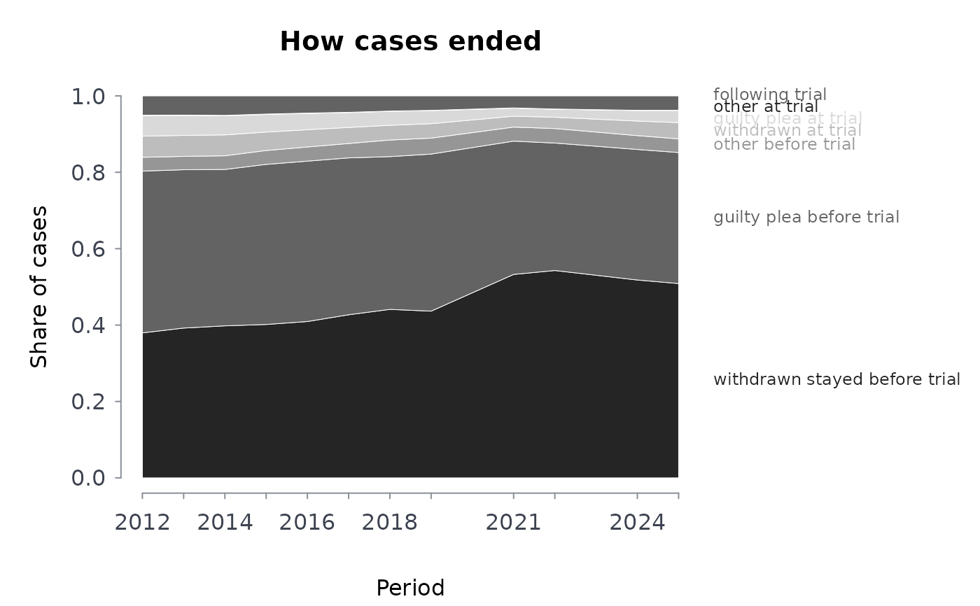
#> ── Outcome shares by period (95% Goodman simultaneous intervals in $shares)
#> Same mix in every period: chi-square 43792.1 on 66 df, p <2e-16, Cramer's V 0.052
#>
#> outcome 2012 2013 2014 2015 2016 2017 2018
#> withdrawn_stayed_before_trial 0.3796 0.3922 0.3980 0.4016 0.4093 0.4270 0.4411
#> guilty_plea_before_trial 0.4236 0.4146 0.4094 0.4191 0.4199 0.4107 0.3999
#> other_before_trial 0.0361 0.0349 0.0358 0.0364 0.0371 0.0377 0.0435
#> withdrawn_at_trial 0.0554 0.0549 0.0547 0.0482 0.0452 0.0421 0.0386
#> guilty_plea_at_trial 0.0536 0.0521 0.0499 0.0462 0.0426 0.0388 0.0366
#> other_at_trial 0.0012 0.0011 0.0012 0.0010 0.0009 0.0007 0.0006
#> following_trial 0.0506 0.0502 0.0510 0.0475 0.0450 0.0430 0.0397
#> 2019 2021 2022 2024 2025
#> 0.4365 0.5326 0.5429 0.5180 0.5088
#> 0.4112 0.3490 0.3338 0.3418 0.3430
#> 0.0418 0.0368 0.0380 0.0362 0.0358
#> 0.0378 0.0286 0.0296 0.0381 0.0426
#> 0.0342 0.0210 0.0209 0.0277 0.0317
#> 0.0006 0.0006 0.0005 0.0005 0.0006
#> 0.0379 0.0315 0.0344 0.0377 0.0376
#> ──────────────────────────────────────────────────────────────────
#> ── Cochran-Armitage trend in each share (Holm-adjusted) ──────────
#> outcome statistic p_value p_holm change
#> withdrawn_stayed_before_trial 29543.56 <2e-16 <2e-16 0.1292
#> guilty_plea_before_trial 10090.69 <2e-16 <2e-16 -0.0806
#> other_before_trial 20.29 6.64e-06 6.64e-06 -0.0003
#> withdrawn_at_trial 3208.77 <2e-16 <2e-16 -0.0128
#> guilty_plea_at_trial 7080.55 <2e-16 <2e-16 -0.0219
#> other_at_trial 187.10 <2e-16 <2e-16 -0.0006
#> following_trial 2172.85 <2e-16 <2e-16 -0.0131
#> ──────────────────────────────────────────────────────────────────
plot(mix)
 # the parts of the result
head(mix$shares)
#> period outcome count total share lower
#> 1 2012 withdrawn_stayed_before_trial 93775 247047 0.3795836 0.3769607
#> 2 2013 withdrawn_stayed_before_trial 90864 231681 0.3921944 0.3894691
#> 3 2014 withdrawn_stayed_before_trial 83626 210098 0.3980333 0.3951641
#> 4 2015 withdrawn_stayed_before_trial 82430 205249 0.4016098 0.3987024
#> 5 2016 withdrawn_stayed_before_trial 84787 207160 0.4092827 0.4063797
#> 6 2017 withdrawn_stayed_before_trial 91440 214137 0.4270163 0.4241433
#> upper
#> 1 0.3822136
#> 2 0.3949265
#> 3 0.4009096
#> 4 0.4045240
#> 5 0.4121920
#> 6 0.4298943
mix$trend
#> outcome statistic p_value p_holm
#> 1 withdrawn_stayed_before_trial 29543.56265 0.000000e+00 0.000000e+00
#> 2 guilty_plea_before_trial 10090.69293 0.000000e+00 0.000000e+00
#> 3 other_before_trial 20.29329 6.643309e-06 6.643309e-06
#> 4 withdrawn_at_trial 3208.77296 0.000000e+00 0.000000e+00
#> 5 guilty_plea_at_trial 7080.54897 0.000000e+00 0.000000e+00
#> 6 other_at_trial 187.10154 1.364671e-42 2.729342e-42
#> 7 following_trial 2172.84508 0.000000e+00 0.000000e+00
#> change
#> 1 0.1292036827
#> 2 -0.0805960172
#> 3 -0.0002635828
#> 4 -0.0127761314
#> 5 -0.0218969033
#> 6 -0.0006064793
#> 7 -0.0130645687
# years as trend scores, so the gap where no row exists is respected
disposition_mix(d[, -(1:2)], period = d$year, scores = d$year)$trend[, 1:3]
#> outcome statistic p_value
#> 1 withdrawn_stayed_before_trial 30150.915355 0.000000e+00
#> 2 guilty_plea_before_trial 10825.914695 0.000000e+00
#> 3 other_before_trial 7.296441 6.909133e-03
#> 4 withdrawn_at_trial 2890.841438 0.000000e+00
#> 5 guilty_plea_at_trial 6782.412494 0.000000e+00
#> 6 other_at_trial 175.420561 4.845824e-40
#> 7 following_trial 2044.569303 0.000000e+00
# outcome columns only: a text column is refused
try(disposition_mix(data.frame(year = c("a", "b"), x = 1:2, y = 3:4)))
#> Error : `counts` has a column that is not numeric (year); pass only the outcome columns
# the parts of the result
head(mix$shares)
#> period outcome count total share lower
#> 1 2012 withdrawn_stayed_before_trial 93775 247047 0.3795836 0.3769607
#> 2 2013 withdrawn_stayed_before_trial 90864 231681 0.3921944 0.3894691
#> 3 2014 withdrawn_stayed_before_trial 83626 210098 0.3980333 0.3951641
#> 4 2015 withdrawn_stayed_before_trial 82430 205249 0.4016098 0.3987024
#> 5 2016 withdrawn_stayed_before_trial 84787 207160 0.4092827 0.4063797
#> 6 2017 withdrawn_stayed_before_trial 91440 214137 0.4270163 0.4241433
#> upper
#> 1 0.3822136
#> 2 0.3949265
#> 3 0.4009096
#> 4 0.4045240
#> 5 0.4121920
#> 6 0.4298943
mix$trend
#> outcome statistic p_value p_holm
#> 1 withdrawn_stayed_before_trial 29543.56265 0.000000e+00 0.000000e+00
#> 2 guilty_plea_before_trial 10090.69293 0.000000e+00 0.000000e+00
#> 3 other_before_trial 20.29329 6.643309e-06 6.643309e-06
#> 4 withdrawn_at_trial 3208.77296 0.000000e+00 0.000000e+00
#> 5 guilty_plea_at_trial 7080.54897 0.000000e+00 0.000000e+00
#> 6 other_at_trial 187.10154 1.364671e-42 2.729342e-42
#> 7 following_trial 2172.84508 0.000000e+00 0.000000e+00
#> change
#> 1 0.1292036827
#> 2 -0.0805960172
#> 3 -0.0002635828
#> 4 -0.0127761314
#> 5 -0.0218969033
#> 6 -0.0006064793
#> 7 -0.0130645687
# years as trend scores, so the gap where no row exists is respected
disposition_mix(d[, -(1:2)], period = d$year, scores = d$year)$trend[, 1:3]
#> outcome statistic p_value
#> 1 withdrawn_stayed_before_trial 30150.915355 0.000000e+00
#> 2 guilty_plea_before_trial 10825.914695 0.000000e+00
#> 3 other_before_trial 7.296441 6.909133e-03
#> 4 withdrawn_at_trial 2890.841438 0.000000e+00
#> 5 guilty_plea_at_trial 6782.412494 0.000000e+00
#> 6 other_at_trial 175.420561 4.845824e-40
#> 7 following_trial 2044.569303 0.000000e+00
# outcome columns only: a text column is refused
try(disposition_mix(data.frame(year = c("a", "b"), x = 1:2, y = 3:4)))
#> Error : `counts` has a column that is not numeric (year); pass only the outcome columns