
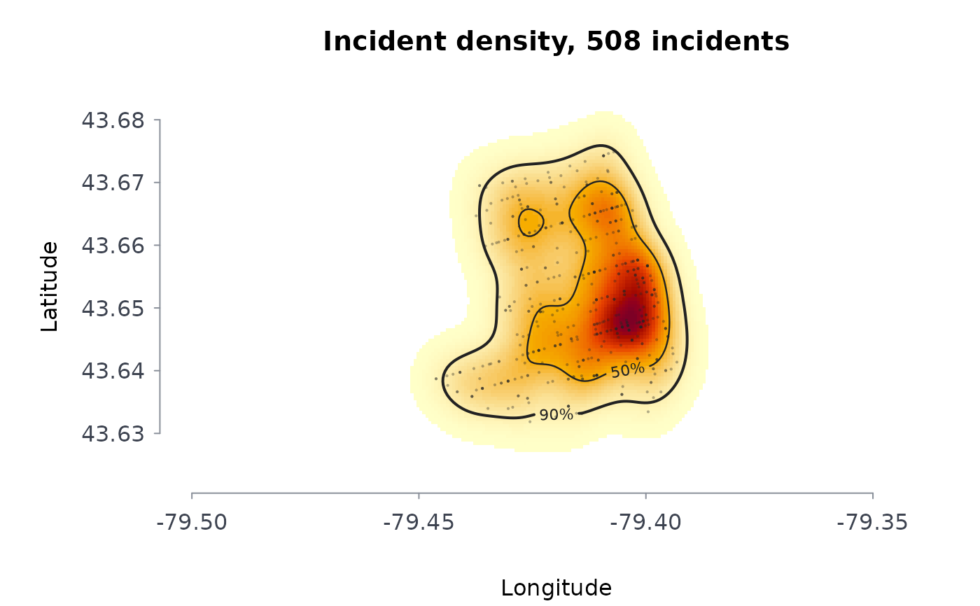
Estimates the density of incident locations – police-reported occurrences, calls for service, addresses of people in a program – as a smooth surface in incidents per square kilometre, and the smallest areas holding a given share of them (the highest-density regions). The plot draws the surface as a heat map with those regions outlined.
Arguments
- lon, lat
Coordinates of the incidents: longitude and latitude in degrees (WGS84) by default, or planar coordinates in metres with
coords = "planar". Points with a missing coordinate are dropped with a message; in degrees, points at exactly (0, 0), which is how several open-data portals publish an incident with no location, are dropped too.- weights
Optional non-negative weight per incident. Default 1.
- bandwidth
Kernel standard deviation in kilometres: one value for both directions or two (east-west, north-south). Default: Scott's normal-reference rule, \(\sigma n^{-1/6}\) for each direction.
- n_grid
Grid nodes per direction. Default 200.
- coverage
Shares of the incidents whose highest-density regions are reported and outlined. Default
c(0.5, 0.9).- coords
"lonlat"(the default) or"planar".
Value
A list of class rmbl_density: field (incidents per
square kilometre on the grid), x and y (grid coordinates
in kilometres from the centre), lon and lat (the same
grid in degrees, for "lonlat"), bandwidth, n,
dropped, points (the projected incidents), and
regions: one row per coverage share with the density
level that bounds it, its area_km2, and its share of the
mapped area.
Details
The estimate is the Gaussian product-kernel density, computed on the grid by linear binning followed by an exact discrete convolution, which agrees with the direct sum to within the binning error (of order the squared grid spacing over the squared bandwidth). The grid extends three bandwidths past the outermost incident so the surface integrates to the total weight.
A highest-density region for share \(p\) is the set of grid cells with the largest densities whose estimated incidents add up to \(p\) of the total. Its area is the spatial counterpart of a concentration index: when half the incidents fall in a few per cent of the mapped area, they are concentrated. The bandwidth decides how sharp the surface is, so it should be reported with any map; the default suits a first look, not a definitive one.
Errors: lon and lat of different lengths, or (with
coords = "lonlat") a coordinate that is not a longitude and
latitude in degrees; fewer than two located incidents with positive weight;
n_grid not a whole number from 10 to 2000; coverage not
shares strictly between 0 and 1; incidents all on one line with no
bandwidth given; a bandwidth that is not one or two positive
numbers, or longer than half the earth's circumference. Incidents with a
missing coordinate are dropped.
References
Scott, D. W. (2015). Multivariate Density Estimation: Theory, Practice, and Visualization, 2nd ed. Wiley, Hoboken, NJ.
Wand, M. P. (1994). Fast computation of multivariate kernel estimators. Journal of Computational and Graphical Statistics, 3(4), 433-445.
Hyndman, R. J. (1996). Computing and graphing highest density regions. The American Statistician, 50(2), 120-126.
Chainey, S., Tompson, L. and Uhlig, S. (2008). The utility of hotspot mapping for predicting spatial patterns of crime. Security Journal, 21(1-2), 4-28.
See also
knox_test, plume_field (the same
kind of surface, for an air pollutant).
Examples
b <- read.csv(system.file("extdata", "tps_break_enter_d14_2024.csv",
package = "rmoriebricklayer"))
kd <- crime_density(b$lon, b$lat, n_grid = 120)
kd
#> ── Kernel density of incidents: smallest areas holding each share
#> 508 incidents; bandwidth 0.337 km east-west, 0.412 km north-south
#> Peak density 77.9 incidents per square kilometre
#>
#> incidents area_km2 share_of_mapped_area density_at_edge
#> 50% 5.506 11.9% 31.91
#> 90% 14.840 32.0% 11.26
#> ──────────────────────────────────────────────────────────────────
plot(kd)
 # a fixed 300 m bandwidth on a coarser grid: a sharper surface
kd3 <- crime_density(b$lon, b$lat, bandwidth = 0.3, n_grid = 60)
kd3$regions
#> coverage level area_km2 area_share
#> 1 0.5 33.66915 5.149953 0.1247222
#> 2 0.9 13.09560 13.763795 0.3333333
# planar coordinates in metres
set.seed(2)
xy <- cbind(rnorm(200, sd = 500), rnorm(200, sd = 500))
crime_density(xy[, 1], xy[, 2], coords = "planar", n_grid = 40)$bandwidth
#> [1] 0.2220670 0.2038706
# longitudes and latitudes are checked
try(crime_density(c(-79.4, 200), c(43.7, 43.8)))
#> Error : coordinate 2 is not a longitude and latitude in degrees (200, 43.8); planar data take coords = "planar"
# a fixed 300 m bandwidth on a coarser grid: a sharper surface
kd3 <- crime_density(b$lon, b$lat, bandwidth = 0.3, n_grid = 60)
kd3$regions
#> coverage level area_km2 area_share
#> 1 0.5 33.66915 5.149953 0.1247222
#> 2 0.9 13.09560 13.763795 0.3333333
# planar coordinates in metres
set.seed(2)
xy <- cbind(rnorm(200, sd = 500), rnorm(200, sd = 500))
crime_density(xy[, 1], xy[, 2], coords = "planar", n_grid = 40)$bandwidth
#> [1] 0.2220670 0.2038706
# longitudes and latitudes are checked
try(crime_density(c(-79.4, 200), c(43.7, 43.8)))
#> Error : coordinate 2 is not a longitude and latitude in degrees (200, 43.8); planar data take coords = "planar"