
What the package is for
crimlab computes statistics that come up again and again in criminology and sociolegal research: disparity measures for policing, the weight of forensic evidence, clearance rates, and what can and cannot be learnt about release rules and sentences from administrative records. It is written for researchers and analysts in criminology, sociolegal studies, policing, corrections and forensic science. Most of the statistics are short formulas. They are easy to get slightly wrong, and easier still to read as showing more than they do.
Each function checks its arguments, computes the quantity in a
compiled core, and returns a plain data frame or named vector. Its help
page says what the number is and the conditions under which it means
what it seems to mean. Where the result rests on an identity or a bound,
proof() names the machine-checked proof of it.
The examples below use made-up numbers chosen to show the arithmetic. None of them is data, and nothing in this vignette is an empirical finding.
Disparities: the veil of darkness
Suppose, purely for illustration, that a force recorded these traffic stops of two groups of drivers, in daylight and in darkness:
day <- c(white = 600, black = 400)
night <- c(white = 700, black = 300)
v <- vodtst(day, night)
v
#>   group   ref shday shnight    ratio sign
#> 1 white  TRUE   0.6     0.7 1.000000   -1
#> 2 black FALSE   0.4     0.3 1.555556    1
pc <- function(x) paste(round(100 * x), "per cent")
Black drivers are 40 per cent of daylight stops and 30 per cent of
stops in darkness. The ratio column compares each group’s
odds of being the one stopped in daylight with its odds in darkness,
against the reference group (the first, here): about 1.56 for black
drivers. The idea, due to Grogger and Ridgeway (2006), is that an
officer can see a driver’s race more easily in daylight, so if race
affects who is stopped, the group it works against makes up a larger
share of daylight stops.
Counts usually come from records, not typed-in vectors. A table of
groups by day and night can be given whole,
and every input is matched by group name, never by position, so the
order in which the groups arrive does not matter; the ref
column marks the reference group:
stops <- data.frame(race = c("black", "white", "white", "black"),
                    light = c("day", "day", "night", "night"),
                    n = c(400, 600, 700, 300))
vodtst(xtabs(n ~ race + light, stops), ref = "white")
#>   group   ref shday shnight    ratio sign
#> 1 black FALSE   0.4     0.3 1.555556    1
#> 2 white  TRUE   0.6     0.7 1.000000   -1
What this does not license: the ratio isolates the effect of
visibility only if the same people are on the road, in the same
proportions, in daylight and in darkness. If black drivers made up a
larger share of daytime traffic than of night-time traffic, the ratio
would exceed 1 with no bias at all. Studies therefore compare stops at
the same clock times in different seasons, when the same commuters drive
in light and in dark. The shift argument shows how much a
difference in exposure would explain. If, say, black drivers’ share of
traffic were 1.3 times as large in daylight as in darkness:
the adjusted ratio is about 1.2. A shift equal to the ratio, about
1.56, would explain the whole contrast. The counts alone cannot tell
bias from a change in who drives; proof("vodtst") names the
theorem that says so.
A related trap is reading an odds ratio as a relative risk. With an outcome as common as 40 per cent, an odds ratio of 3 corresponds to a much smaller relative risk:
r <- orrisk(or = 3, rate = 0.4, share = 0.5)
r
#>   exposed unexposed        rr        or
#> 0.5282202 0.2717798 1.9435596 3.0000000
The relative risk is 1.94, not 3.
Forensics: a match and what it is worth
Take a DNA profile typed at two loci, heterozygous at the first and homozygous at the second, with these (illustrative) allele frequencies and a coancestry coefficient of 0.03:
m <- gtmp(p = c(D3 = 0.1, vWA = 0.2), q = c(0.3, NA),
          hom = c(FALSE, TRUE), theta = 0.03)
m
#> $locus
#>   locus   hom         mp
#> 1    D3 FALSE 0.07467851
#> 2   vWA  TRUE 0.06607071
#>
#> $log10mp
#> [1] -2.306795
#>
#> $log10lr
#> [1] 2.306795
10^m[["log10lr"]]
#> [1] 202.6728
The match probability is the chance that an unrelated person from the same population would share the profile. Its reciprocal, about 200 here, is the likelihood ratio for a single-source match: the profile is that many times as probable if the suspect is the source as if an unrelated person is.
What this does not license: a likelihood ratio is not the probability that the suspect is the source. That needs a prior, and the same ratio gives very different answers under different priors:
lrpost(lr = rep(10^m[["log10lr"]], 3), prior = c(1 / 10, 1 / 1000, 1 / 1e5))
#> [1] 0.957481538 0.168658859 0.002022648
Reading the ratio as the posterior is the prosecutor’s fallacy. The
ratio also assumes the alternative source is unrelated to the suspect. A
brother is far more likely to share the profile; kinidx()
gives the weight of two profiles for a stated relationship.
How good is a system that reports likelihood ratios? Given ratios
from validation comparisons whose truth is known, the
log-likelihood-ratio cost scores them, in bits: 1 for a system that
always reports 1, and close to 0 for one that separates the two kinds of
comparison perfectly with ratios far from 1. cllrmin()
recalibrates the ratios with the pool-adjacent-violators algorithm,
which keeps their order, and splits the cost into the cost after
recalibration (min) and the rest (cal):
same <- c(50, 200, 8, 0.5)
diff <- c(0.01, 0.2, 1.5, 0.001)
cm <- cllrmin(same, diff)
cm
#>      cllr       min       cal
#> 0.4239265 0.2500000 0.1739265
With these made-up ratios one different-source ratio (1.5) is larger
than one same-source ratio (0.5), so recalibration cannot remove all the
cost: 0.25 bits remain after it, and the other 0.17 come from the ratios
being too large or too small for what they separate. That no
order-keeping recalibration could do better than the
pool-adjacent-violators one is the usual reading of min,
but it is not among the theorems proof("cllrmin") names.
With four comparisons of each kind this says nothing about any real
system; validation needs many comparisons, made under the conditions of
casework. A Tippett plot shows the same ratios as two curves:
tipplt(same, diff)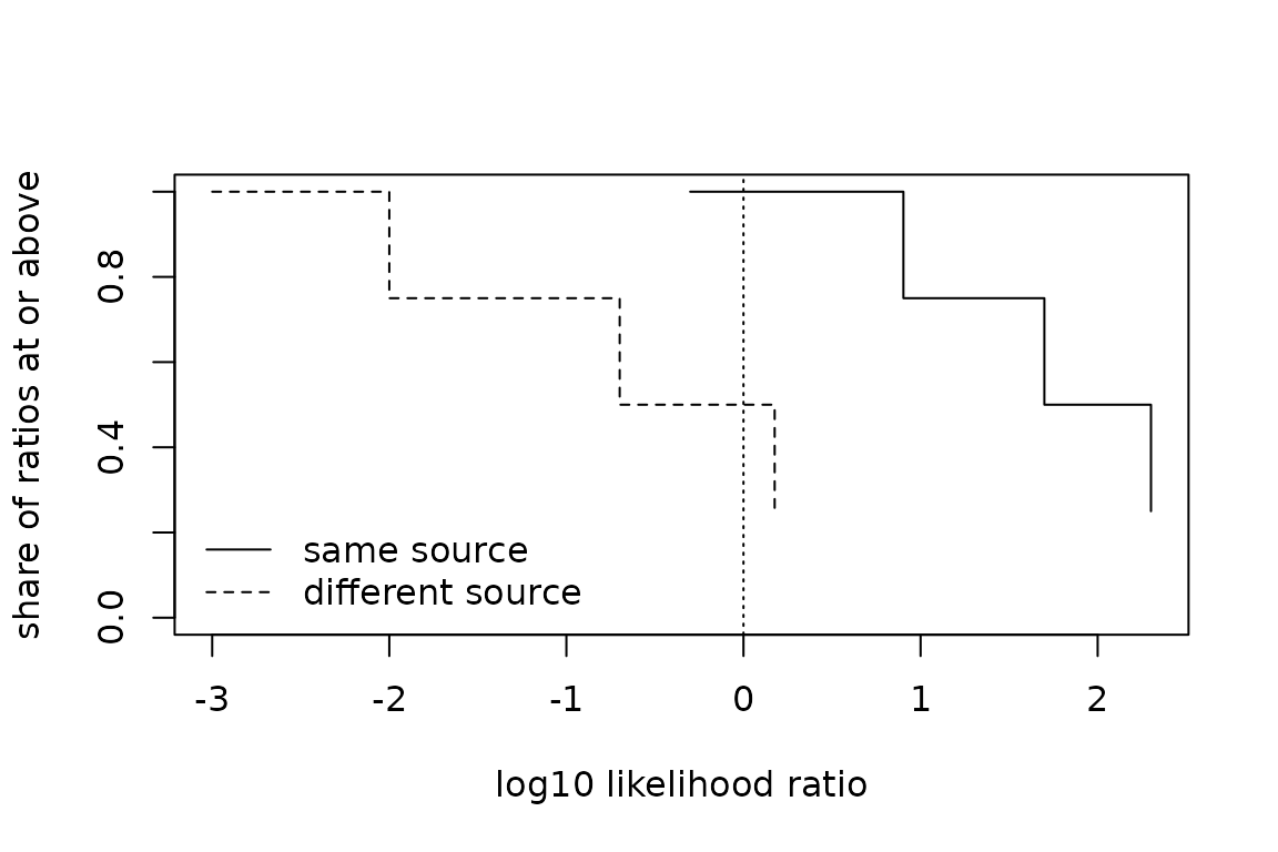
Policing: clearance rates and Simpson’s paradox
Two (invented) years of offences recorded and cleared, by type:
cl <- clrsmp(clra = c(minor = 90, serious = 20),
             reca = c(minor = 100, serious = 50),
             clrb = c(minor = 19, serious = 60),
             recb = c(minor = 20, serious = 140))
cl[["parts"]]
#>      part ratea     rateb    sharea shareb    rateeff     mixeff
#> 1   minor   0.9 0.9500000 0.6666667  0.125 0.01979167 -0.1687066
#> 2 serious   0.4 0.4285714 0.3333333  0.875 0.01726190 -0.1079303
tot <- cl[["total"]]
tot
#>       ratea       rateb      change     rateeff      mixeff          up
#>  0.73333333  0.49375000 -0.23958333  0.03705357 -0.27663690  2.00000000
#>        down     simpson
#>  0.00000000  2.00000000
Both types clear better in year B than in year A, yet the aggregate
rate falls from about 0.73 to about 0.49. The decomposition shows why:
the rate effect is positive, and the mix effect is negative and larger
than the fall, because recorded work moved toward serious offences,
which clear less often. simpson is 2 because every type
moved one way and the aggregate the other.
What this does not license: the decomposition is arithmetic on the recorded counts. It says nothing about whether the service worked better or worse. Clearance depends on what is recorded, how offences are classified, and what counts as cleared, and any of these can change between years or between services. An aggregate clearance rate compared without the split by type can point the wrong way, as here; the split by type is only as good as the classification.
Corrections: what records say about a sentence
Suppose (again for illustration) 500 people, each given a community sentence or custody, with an indicator of reconviction:
set.seed(1)
z <- sample(c("community", "custody"), 500, replace = TRUE,
            prob = c(0.6, 0.4))
y <- rbinom(500, 1, ifelse(z == "custody", 0.55, 0.35))
sb <- sntbnd(y, z, treat = "custody")
sb
#>        term share  lower upper  observed
#> 1 community 0.624  0.208 0.584 0.3333333
#> 2   custody 0.376  0.192 0.816 0.5106383
#> 3    effect    NA -0.392 0.608 0.1773050
The observed reconviction rates differ by about 0.18. But each person is seen under one sentence only. Without assumptions about who receives which sentence, the reconviction rate everyone would have had under custody is known only to lie within an interval as wide as the share who did not receive custody, and the effect of custody against a community sentence lies in an interval of width exactly 1 that contains 0 (Manski and Nagin 1998).
What this does not license: the observed difference is not the effect of the sentence. Judges choose sentences with information about the person, so the two groups differ before sentencing. Narrowing the interval needs an assumption that the data cannot check, such as random assignment, and the conclusions are only as good as that assumption.
Networks: who offends with whom
Police records list the offenders of each incident. Joining offenders who were recorded together gives a co-offending network, the tie weighted by the incidents they share (Reiss 1988):
inc <- c(1, 1, 1, 2, 2, 3, 3, 4, 4, 5, 5, 6)
off <- c("ana", "ben", "cy", "ana", "ben", "cy", "dee", "dee", "eli",
         "eli", "fay", "gus")
g <- coofg(inc, off)
e <- g$edges
e
#>   from  to w
#> 1  ana ben 2
#> 2  ana  cy 1
#> 3  ben  cy 1
#> 4   cy dee 1
#> 5  dee eli 1
#> 6  eli fay 1
Gus offended alone: he is a node of the network but in no tie, so the
network functions are given nodes to keep him. Results come
back by name, in the order offenders first appear:
ntdeg(e$from, e$to, w = e$w, nodes = g$nodes)
#>   node deg wdeg
#> 1  ana   2    3
#> 2  ben   2    3
#> 3   cy   3    3
#> 4  dee   2    2
#> 5  eli   2    2
#> 6  fay   1    1
#> 7  gus   0    0
ntbtw(e$from, e$to, nodes = g$nodes)
#>   node btw
#> 1  ana   0
#> 2  ben   0
#> 3   cy   6
#> 4  dee   6
#> 5  eli   4
#> 6  fay   0
#> 7  gus   0
ntlvn(e$from, e$to, w = e$w, nodes = g$nodes)$memb
#>   node comm
#> 1  ana    1
#> 2  ben    1
#> 3   cy    1
#> 4  dee    2
#> 5  eli    2
#> 6  fay    2
#> 7  gus    3
Cy and Dee each lie on every path between the two halves, and the
Louvain method splits the network there. ntchg() measures
how cleanly it splits: the conductance of the best cut lies between the
two Cheeger bounds, and the lower one is proved in Lean
(proof("ntchg")).
big <- !(e$from == "gus" | e$to == "gus")
ntchg(e$from[big], e$to[big], w = e$w[big])$bound
#>    lambda2      lower      upper      sweep
#> 0.17307222 0.08653611 0.58834041 0.20000000
What this does not license: a recorded tie is two people arrested or charged for the same incident, so the network shows police attention as much as offending. Offenders never caught are missing, and a missing node can change who appears central; betweenness in particular is fragile when ties are missing.
Places: where incidents are and how they spread
Thirty (simulated) burglaries around two centres, in metres on a local grid:
set.seed(2)
xy <- data.frame(x = c(rnorm(20, 1000, 120), rnorm(10, 1800, 60)),
                 y = c(rnorm(20, 2000, 80), rnorm(10, 2300, 60)))
cs <- cgstat(xy)
cs[c("mx", "my", "sdd")]
#>        mx        my       sdd
#> 1288.2054 2095.6282  434.9568
el <- sdell(xy, c = 2)
el
#>           mx           my            a            b        angle         area
#> 1.288205e+03 2.095628e+03 8.486237e+02 1.912781e+02 3.682120e-01 5.099533e+05
The mean centre summarises where the incidents are and the standard
distance deviation how far they spread, about 435 metres. The ellipse
with c = 2 would hold about 86 per cent of bivariate normal
points; here the points are two clusters, so the ellipse describes their
joint spread, not a shape that any cluster has.
nn <- nnidx(xy, win = c(500, 2300, 1600, 2700), nsim = 99, seed = 1)
nn$order[, c("mean", "exp", "ratio", "pclu")]
#>      mean      exp     ratio pclu
#> 1 53.9421 128.4523 0.4199387 0.01
The mean nearest-neighbour distance is well below its expectation under complete spatial randomness in the study rectangle, and the Monte Carlo p-value against clustering is small. What this does not license: the expectation depends on the rectangle chosen. A rectangle drawn around the points makes them look less clustered than one covering the whole area at risk, and neither says why the incidents cluster; burglaries follow housing, which is itself clustered.
Risk tools: one score, several kinds of fairness
A (simulated) risk score for 400 people in two groups whose base rates differ:
set.seed(3)
g <- rep(c("a", "b"), each = 200)
y <- rbinom(400, 1, ifelse(g == "a", 0.3, 0.5))
s <- plogis(rnorm(400, ifelse(y == 1, 0.8, -0.8)))
fm <- fair(s, y, g, cut = 0.5)
fm$met[, c("group", "fpr", "fnr", "ppv")]
#>   group       fpr       fnr       ppv
#> 1     a 0.1702128 0.1864407 0.6666667
#> 2     b 0.2371134 0.2330097 0.7745098
The score is the same function of the outcome in both groups, yet the false positive rates and the predictive values differ, because the base rates do. What this does not license: no single row of this table is “the” fairness of the tool. When base rates differ, equal error rates and equal predictive values cannot all hold at once (Chouldechova 2017); which to equalise is a choice about whose errors matter, not a statistical finding.
Proofs
proof() lists the theorems behind a function:
p <- proof("clrsmp")
p
#>       fn                                 theorem                file
#> 1 clrsmp       Crimlab.Clearance.agg_eq_weighted lean/Clearance.lean
#> 2 clrsmp              Crimlab.Clearance.kitagawa lean/Clearance.lean
#> 3 clrsmp         Crimlab.Clearance.change_ge_mix lean/Clearance.lean
#> 4 clrsmp Crimlab.Clearance.fixed_mix_no_reversal lean/Clearance.lean
#> 5 clrsmp       Crimlab.Clearance.simpson_witness lean/Clearance.lean
The files ship with the package and can be read in R or checked with Lean (see the README). This is the statement of Kitagawa’s identity, the reason the rate and mix effects always add up to the change:
src <- readLines(system.file(p[["file"]][1], package = "crimlab"),
                 encoding = "UTF-8")
i <- grep("^theorem kitagawa", src)
writeLines(src[i:(i + 2)])
#> theorem kitagawa (wa wb ra rb : ι → ℝ) (c : ℝ) (ha : ∑ k, wa k = 1) (hb : ∑ k, wb k = 1) :
#>     ∑ k, wb k * rb k - ∑ k, wa k * ra k =
#>       ∑ k, (wa k + wb k) / 2 * (rb k - ra k) + ∑ k, ((ra k + rb k) / 2 - c) * (wb k - wa k) := by
A Lean proof guarantees that the theorem, exactly as stated, follows from its hypotheses over the real numbers. It does not guarantee three other things:
- that the code is free of bugs. The C++ core uses floating-point arithmetic, not real numbers, and could compute something other than the formula proved. The package’s tests check the code against the proved identities, which is evidence, not proof;
- that the statement is the one you need. Read it: a theorem about workload shares that sum to 1 says nothing about shares that do not;
- that your data meet the model’s assumptions. The veil-of-darkness theorem holds when exposure is the same in daylight and darkness; whether it is for a given force and year is a question about the world, not about the proof.
References
Chouldechova, A. (2017). Fair prediction with disparate impact: a study of bias in recidivism prediction instruments. Big Data, 5(2), 153-163.
Grogger, J. and Ridgeway, G. (2006). Testing for racial profiling in traffic stops from behind a veil of darkness. Journal of the American Statistical Association, 101(475), 878-887.
Kitagawa, E. M. (1955). Components of a difference between two rates. Journal of the American Statistical Association, 50(272), 1168-1194.
Manski, C. F. and Nagin, D. S. (1998). Bounding disagreements about treatment effects: a case study of sentencing and recidivism. Sociological Methodology, 28(1), 99-137.
Reiss, A. J. (1988). Co-offending and criminal careers. Crime and Justice, 10, 117-170.