
Compare rated scales (perceived mental health, life satisfaction) between groups
Source:R/indigenous_mental_health.R
ordcmp.RdFor a rated scale published as the percentage in each category with its confidence limits (perceived mental health from poor to excellent, life satisfaction from 0 to 10, agreement with a statement), the probability that a person in each group rates higher than a person in the reference group, with its confidence interval: a comparison of the whole distribution, not of one category cut from it.
Usage
ordcmp(
  data,
  grp,
  cat,
  est,
  lower,
  upper,
  lvls,
  ref,
  qual = NULL,
  conflvl = 0.95,
  pooled = NULL
)
Arguments
- data
A data frame, one row per group and category (as
scestsgives, filtered to one geography, age group and gender).- grp, cat, est, lower, upper
Column names: the group, the category, the share in it (percent or proportion: only relative shares matter) and its published limits on the same scale.
- lvls
The categories, from the lowest (least favourable) to the highest.
- ref
The label of the reference group (required: any group of
data).- qual
Optional column of quality flags (see
qltyrcd).- conflvl
Confidence level of the published limits and of the result (default 0.95).
- pooled
Optional labels of rows that pool other groups (see
indgap).
Value
A data frame of class rmbl_ordinal_compare: group,
reference, probbet, lower, upper, delta,
neff, neffref, usewithcau, poogrp; the
attribute shares is the matrix of shares (groups by levels), which
plot() draws.
Details
With shares \(p_i\) in the group and \(q_j\) in the reference over categories ordered from lowest to highest, the probability of a higher rating, ties counted half, is \(A = \sum_i p_i (Q_{i-1} + q_i / 2)\) with \(Q_i\) the reference's cumulative shares and \(Q_0 = 0\): the Mann-Whitney probability, equal to \(\alpha / (1 + \alpha)\) for Agresti's (1980) generalized odds ratio \(\alpha\) with ties split equally, and to the mean ridit of the group with the reference as the standard (Bross 1958). 0.5 is no difference; \(2A - 1\) is Cliff's \(\delta\), the share rating higher less the share rating lower.
Its variance is that of the two-sample U statistic, \(\sigma_1^2 / n_1 + \sigma_0^2 / n_0\), with \(\sigma_1^2\) the variance over the group of each category's placement in the reference and \(\sigma_0^2\) the converse (Brunner and Munzel 2000). The sample sizes are the effective ones the published limits imply: for each category, \(n = p(1 - p) / s^2\) with \(s\) the standard error from the limits' width, taking the median over the categories. That carries the design effect of the survey's weights and clusters, which the counts of persons (population totals) do not. The interval is built on the logit scale, so it stays inside 0 and 1.
The categories given in lvls are taken as the whole scale: rows for
totals, for combined categories (“Excellent or very good”) and for
“not specified” are left out, and the shares are rescaled to sum to
one over the levels. A group with a suppressed or missing category is not
compared, since its distribution is unknown; one with an E category
(in the group or the reference) is compared and marked, and one whose
published interval misses its own estimate is not compared.
A higher rating means better only on a scale that runs that way. Give
lvls from the least to the most favourable so that probbet
reads as its name says.
References
Agresti A (1980). Generalized odds ratios for ordinal data. Biometrics 36(1):59-67. doi:10.2307/2530495
Bross IDJ (1958). How to use ridit analysis. Biometrics 14(1):18-38. doi:10.2307/2527727
Brunner E, Munzel U (2000). The nonparametric Behrens-Fisher problem: asymptotic theory and a small-sample approximation. Biometrical Journal 42(1):17-25. doi:10.1002/(SICI)1521-4036(200001)42:1<17::AID-BIMJ17>3.0.CO;2-U
Examples
# Self-perceived mental health, 15 years and older, Canada, 2022 (table
# 41-10-0067-01)
mh <- indiex("mentalhealth")
mh <- mh[mh$region == "Canada", ]
oc <- ordcmp(
mh,
"group",
"rating",
"estimate",
"lower",
"upper",
lvls = c("Fair or poor", "Good", "Very good", "Excellent"),
ref = "M\u00e9tis",
qual = "quality"
)
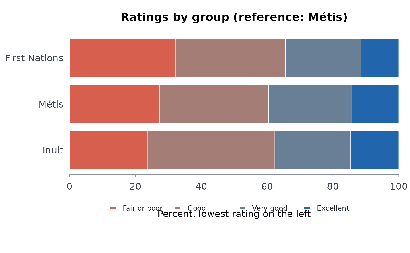
oc
#> ╭── Ordinal comparison against a reference group ────────────────────────╮
#> │ Reference Métis │
#> │ Reference neff 3,884 │
#> │ Levels 4 │
#> │ Measure chance a person in the group rates higher, ties half │
#> │ │
#> │ group probbet 95% CI delta neff │
#> │ ------------- ------- -------------- -------- ----- │
#> │ First Nations 0.4653 [0.453, 0.477] -0.06940 4,021 │
#> │ Inuit 0.5062 [0.493, 0.520] 0.01247 2,792 │
#> │ │
#> │ Rate lower than Métis (interval below 0.5): First Nations. │
#> │ Not distinguishable from 0.5 (interval includes it): Inuit. │
#> │ │
#> │ probbet 0.5 is no difference; above 0.5 the group rates higher. │
#> │ delta (Cliff's) = share rating higher less share rating lower. │
#> │ neff: the effective sample size the published limits imply (it │
#> │ carries the survey's design effect). │
#> ╰────────────────────────────────────────────────────────────────────────╯
plot(oc)
 # your own table: a made-up four-level rating for two groups, with limits
own <- data.frame(
group = rep(c("Nation A", "Everyone else"), each = 4),
rating = rep(c("Poor", "Fair", "Good", "Excellent"), 2),
pct = c(10, 25, 40, 25, 6, 20, 44, 30),
lo = c(7, 21, 35, 21, 5, 18, 42, 28),
hi = c(13, 29, 45, 29, 7, 22, 46, 32)
)
ordcmp(own, "group", "rating", "pct", "lo", "hi",
lvls = c("Poor", "Fair", "Good", "Excellent"), ref = "Everyone else")
#> ╭── Ordinal comparison against a reference group ────────────────────────╮
#> │ Reference Everyone else │
#> │ Reference neff 2,092 │
#> │ Levels 4 │
#> │ Measure chance a person in the group rates higher, ties half │
#> │ │
#> │ group probbet 95% CI delta neff │
#> │ -------- ------- -------------- ------- ---- │
#> │ Nation A 0.4475 [0.419, 0.477] -0.1050 417 │
#> │ │
#> │ Rate lower than Everyone else (interval below 0.5): Nation A. │
#> │ │
#> │ probbet 0.5 is no difference; above 0.5 the group rates higher. │
#> │ delta (Cliff's) = share rating higher less share rating lower. │
#> │ neff: the effective sample size the published limits imply (it │
#> │ carries the survey's design effect). │
#> ╰────────────────────────────────────────────────────────────────────────╯