Hawkes processes: self-exciting event series • rmoriebricklayer

Many administrative event series cluster: one incident raises the chance of another soon after. A Hawkes process (Hawkes 1971) models this directly. Its conditional intensity, the instantaneous event rate given the past, is

$\lambda(t) = \mu + \sum_{t_i < t} \phi(t - t_i),$

a baseline rate $\mu$ plus a kernel $\phi$ that each past event adds and that decays with the time since it. The integral of the kernel, $n = \int_0^\infty \phi(s)\,ds$ , is the branching ratio: the expected number of events each event directly triggers. When $n < 1$ the process is stationary; $n$ is the fraction of events that are “children” of earlier events rather than arrivals from the baseline, which is often the quantity of substantive interest.

Simulating a Hawkes process

Ogata’s thinning algorithm simulates the process exactly: propose events from an upper bound on the intensity and keep each with probability $\lambda(t)/\lambda_{\max}$ . Here is an exponential kernel $\phi(s) = \alpha \beta e^{-\beta s}$ , whose branching ratio is $\alpha$ :

simulate_hawkes <- function(mu, alpha, beta, horizon, seed = 1) {
  set.seed(seed)
  t <- 0
  events <- numeric(0)
  while (t < horizon) {
    lambda_max <- mu + alpha * beta * sum(exp(-beta * (t - events)))
    t <- t + stats::rexp(1, lambda_max)
    if (t >= horizon) break
    lambda_t <- mu + alpha * beta * sum(exp(-beta * (t - events)))
    if (stats::runif(1) <= lambda_t / lambda_max) events <- c(events, t)
  }
  events
}
times <- simulate_hawkes(mu = 1, alpha = 0.5, beta = 2, horizon = 300)
length(times)
#> [1] 559

Fitting

core_hawkes_fit() maximises the exact log-likelihood with an analytic gradient in C (projected BFGS, with the parameters bounded). theta holds the baseline, the branching ratio and the kernel parameter:

fit <- core_hawkes_fit(times, horizon = 300, kernel = "exponential")
fit$theta
#> [1] 0.1027148 0.4073514 2.1590220
fit$branching_ratio
#> [1] 0.4073514

The branching ratio is recovered close to the 0.5 the data were simulated with, and the baseline close to 1. Four kernels are available: exponential (memoryless decay), weibull and gamma (a delayed peak), lomax (a heavy tail: influence that fades slowly). Compare them by information criterion:

sapply(c("exponential", "weibull", "lomax"), function(k) {
  core_hawkes_fit(times, 300, kernel = k)$aic
})
#> exponential     weibull       lomax 
#>    352.1139    353.6296    354.1802

A sinusoidal baseline lets the background rate follow a cycle (a weekly or seasonal pattern) instead of staying constant:

core_hawkes_fit(times, 300, kernel = "exponential", baseline = "sinusoidal")$aic
#> [1] 352.3058

Checking the fit: time-rescaling residuals

If the fitted intensity is right, the compensator $\Lambda(t_i) = \int_0^{t_i}\lambda(s)\,ds$ turns the event times into a unit-rate Poisson process (the time-rescaling theorem; Brown et al. 2002). core_hawkes_residuals() returns the rescaled inter-event quantities, which should then be uniform:

U <- core_hawkes_residuals(times, 300, "exponential", fit$theta)
stats::ks.test(U, "punif")$p.value
#> [1] 0.8168762

plot(stats::qunif(stats::ppoints(length(U))), sort(U), pch = 20, cex = .6,
     xlab = "uniform quantiles", ylab = "rescaled residuals",
     main = "Time-rescaling check")
abline(0, 1, col = 2)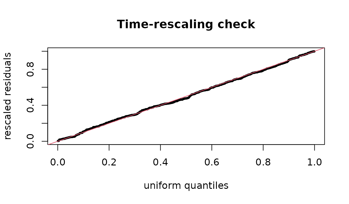

A misspecified kernel shows as a departure from the diagonal; a p-value well below 0.05 says the model does not explain the clustering it was fitted to.

Events recorded to a resolution

Administrative data record dates, not instants. Many events on one day are ties, and a Hawkes likelihood with tied times is ill-defined (the kernel at lag zero). core_hawkes_jitter() spreads each day’s events uniformly across that day, deterministically from a seed, so the fit is reproducible and no two events coincide:

days <- c(0, 0, 0, 1, 3, 3)
core_hawkes_jitter(days)
#> [1] 0.1599104 0.2786011 0.7415649 1.3441907 3.0380302 3.8682281
anyDuplicated(core_hawkes_jitter(days))
#> [1] 0

Fit on jittered times, and treat the day as the unit of the horizon.

Evaluating a likelihood directly

core_hawkes_nll() returns the negative log-likelihood at given parameters, for profile plots, likelihood-ratio comparisons or a check against another implementation:

core_hawkes_nll(times, 300, "exponential", fit$theta)
#> [1] 173.0569
core_hawkes_nll(times, 300, "exponential", fit$theta * 1.5)
#> [1] 193.815

Boundaries and identifiability

A heavy-tailed kernel that tends to its exponential limit has a shape parameter that is not identified; the fit then stops at the parameter bound and says so (fit$at_bound), instead of reporting an absurd estimate. Short series carry little information about the kernel’s shape: with a few hundred events, compare kernels by AIC but do not read much into the third decimal of a shape parameter.

References

Hawkes (1971). Spectra of some self-exciting and mutually exciting point processes. Biometrika 58(1). Ogata (1981). On Lewis’ simulation method for point processes. IEEE Trans. Inf. Theory. Brown, Barbieri, Ventura, Kass, Frank (2002). The time-rescaling theorem and its application to neural spike train data analysis. Neural Computation 14(2).