Time-rescaling residuals of a Hawkes process

Transforms the event times into residuals that are independent and uniform on (0, 1) when the fitted Hawkes model is right, by the time-rescaling theorem. Plot them, or test them against the uniform with stats::ks.test(), to check the fit of core_hawkes_fit(); departures show where the model misses clustering or a trend.

Usage

core_hawkes_residuals(
  times,
  horizon,
  kernel = c("exponential", "weibull", "gamma", "lomax"),
  par,
  baseline = c("constant", "sinusoidal")
)

Arguments

times

Numeric vector of event times, sorted increasingly, all in [0, horizon], in any time unit (days are the natural unit for the sinusoidal baseline's yearly cycle). At least 50 events.

horizon

End of the observation window, one positive number in the same unit as times; the window is [0, horizon].

kernel

The triggering kernel: "exponential" (the default), "weibull", "gamma" or "lomax".

par

Numeric vector of parameters (baseline terms, eta, kernel parameters), as core_hawkes_fit() returns them in theta: length 3 for the exponential kernel with a constant baseline, one more for a two-parameter kernel, three more for the sinusoidal baseline.

baseline

"constant" (the default) or "sinusoidal" (trend plus a 365.25-unit cycle).

Value

A numeric vector of length length(times), values in (0, 1).

Details

With the compensator \(\Lambda(t) = \int_0^t \lambda(s)\,ds\), the residual of event \(i\) is $$U_i = 1 - \exp(-(\Lambda(t_i) - \Lambda(t_{i-1})))$$ with \(t_0 = 0\) (Brown et al. 2002). The rescaled gaps \(\Lambda(t_i) - \Lambda(t_{i-1})\) are unit-rate exponential under the model, so the \(U_i\) are uniform. The model and kernels are those of core_hawkes_fit(); the shared C++ core computes the residuals in O(n) for the exponential kernel and O(n w) for the others. Tied times give tied residuals.

Errors: times with NA, unsorted or outside [0, horizon]; par of the wrong length (2 + kernel parameters for the constant baseline, 5 + kernel parameters for the sinusoidal one).

References

Brown EN, Barbieri R, Ventura V, Kass RE, Frank LM (2002). The time-rescaling theorem and its application to neural spike train data analysis. Neural Comput. 14, 325–346. doi:10.1162/08997660252741149

Examples

set.seed(2)
times <- sort(stats::runif(200, 0, 50))
U <- core_hawkes_residuals(times, 50, "exponential", c(log(3), 0.2, 2))
stats::ks.test(U, "punif")$p.value
#> [1] 0.7935876

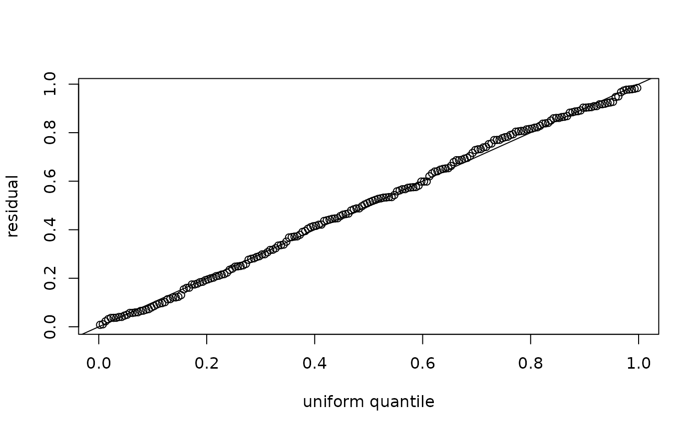
# residuals of a fitted model, and a quick uniform Q-Q check
fit <- core_hawkes_fit(times, 50, "weibull")
U2 <- core_hawkes_residuals(times, 50, "weibull", fit$theta)
summary(U2)
#>     Min.  1st Qu.   Median     Mean  3rd Qu.     Max. 
#> 0.008058 0.245728 0.511733 0.503234 0.778263 0.984104 
plot(stats::ppoints(length(U2)), sort(U2), xlab = "uniform quantile", ylab = "residual")
abline(0, 1)


# par must match the kernel and baseline
try(core_hawkes_residuals(times, 50, "weibull", c(log(3), 0.2, 2)))
#> Error : `par` must have length 4