Hawkes process: time-rescaling residuals

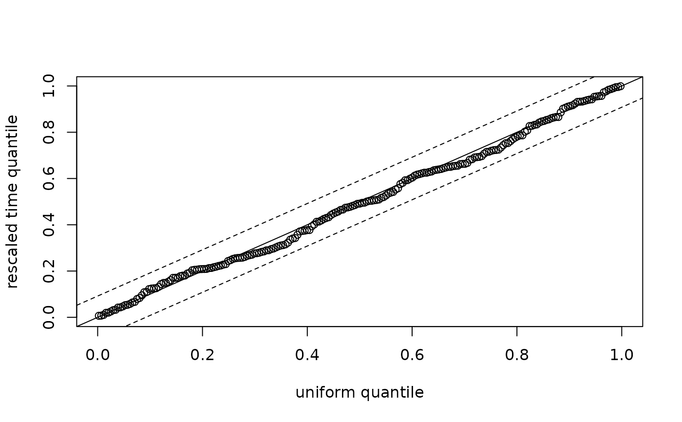
Transforms event times by the compensator of a Hawkes process, \(\Lambda(t) = \int_0^t \lambda\): under the model the gaps \(\tau_i = \Lambda(t_i) - \Lambda(t_{i-1})\) (with \(t_0 = 0\)) are independent standard exponentials, so u = 1 - exp(-tau) are uniform on [0, 1]. The Kolmogorov-Smirnov test compares u with the uniform, with R's exact p-value below 100 events without ties and the limiting distribution otherwise, as stats::ks.test() does. plot() draws the uniform quantile plot with the test's 95% band.

Usage

hwkres(
  times,
  hor = NULL,
  par = NULL,
  kernel = "exp",
  base = "const",
  per = 365.25
)

# S3 method for class 'hwkres'
plot(x, ...)

Arguments

times

A fit from hwkfit(), or event times as there.

hor, kernel, base, per

As for hwkfit() (not read with a fit); one kernel and one baseline.

par

The parameters, as par of hwkfit() (not read with a fit).

x

An hwkres object.

...

Passed to graphics::plot().

Value

An object of class hwkres, a list: tau, the rescaled gaps; u, their uniform transforms; d and p, the Kolmogorov-Smirnov statistic and p-value; and n.

References

Ogata, Y. (1988). Statistical models for earthquake occurrences and residual analysis for point processes. Journal of the American Statistical Association, 83(401), 9-27. doi:10.1080/01621459.1988.10478560

Examples

x <- hwksim(c(a0 = log(0.5), eta = 0.5, beta = 2), 200, seed = 1)
r <- hwkres(hwkfit(x$t, 200))
r
#> hwkres: 219 rescaled gaps, mean 0.9965042 (1 under the model)
#> Kolmogorov-Smirnov D 0.04543387, p 0.7566163
plot(r)