
A weighted average of untreated units that tracks the treated unit before the policy, as its counterfactual after; with the placebo test that runs the same method on every untreated unit.
Value
A list of class rmbl_synth: weights (a named vector
over the donors), path (a data frame: time, treated,
synthetic, gap), rmspepre, rmsperatio,
p_value (NA without the placebo), placrat.
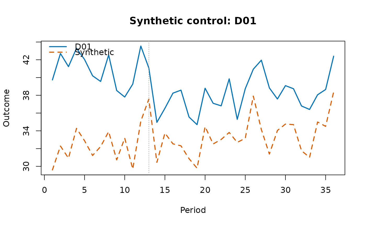
plot() draws the two paths and the gap.
Details
The weights solve $$\min_w \sum_{t < T_0} \Big(Y_{1t} - \sum_j w_j Y_{jt}\Big)^2 \quad \textrm{s.t.} \quad w_j \ge 0,\ \sum_j w_j = 1,$$ over the periods before adoption \(T_0\) (accelerated projected gradient onto the simplex; the problem is convex, so the solution is the global one). The effect in each period is the gap \(Y_{1t} - \sum_j w_j Y_{jt}\). For inference, each untreated unit in turn is treated as if it had adopted the policy, with the other untreated units as donors; the ratio of root mean squared gap after to before adoption ranks the real unit among the placebos, and \(p\) is its rank over the number of units (Abadie, Diamond and Hainmueller 2010).
This version matches on the pre-period outcomes only, not on separate predictors.
References
Abadie A, Diamond A, Hainmueller J (2010). Synthetic control
methods for comparative case studies. Journal of the American Statistical
Association 105(490):493-505.
doi:10.1198/jasa.2009.ap08746
Examples
p <- polex()
p1 <- p[is.na(p$refmonth) | p$district == "D01", ]
s <- synctl(p1, "district", "month", "crmrate", treunit = "D01",
adopt = 13)
round(s$weights, 3)
#> D04 D08 D12 D16 D20
#> 0 1 0 0 0
s$p_value
#> [1] 1
plot(s)
 # your own panel: eight towns over ten years, four adopting a by-law (two
# in 2019, two in 2021), with each town's population, county and income
own <- data.frame(
town = rep(c("A", "B", "C", "D", "E", "F", "G", "H"), each = 10),
year = rep(2015:2024, times = 8)
)
i <- match(own$town, unique(own$town))
own$first <- c(2019, 2019, 2021, 2021, NA, NA, NA, NA)[i]
own$bylaw <- as.integer(!is.na(own$first) & own$year >= own$first)
own$pop <- c(12, 30, 8, 22, 15, 40, 9, 18)[i] * 1000
own$county <- rep(c("North", "South"), 4)[i]
own$income <- 50 + own$year - 2015 + cos(seq_len(80))
own$rate <- 30 + i + 0.5 * (own$year - 2015) - 4 * own$bylaw +
0.2 * own$income + sin(seq_len(80))
# one treated town, A, against the four towns never treated
own1 <- own[is.na(own$first) | own$town == "A", ]
synctl(own1, "town", "year", "rate", treunit = "A", adopt = 2019)
#> ╭── Synthetic control ────────────────────────────────────────────────────╮
#> │ Treated unit A │
#> │ Adoption 2019 │
#> │ Donors 4 │
#> │ Donors with weight 1 │
#> │ Pre-period RMSPE 3.507 │
#> │ Mean gap after -7.923 │
#> │ Post/pre RMSPE ratio 2.29 │
#> │ Placebo-in-space p 0.200 │
#> │ Placebos 4 │
#> │ │
#> │ Donor weights │
#> │ donor weight │
#> │ ----- ------ │
#> │ E 1 │
#> │ │
#> │ The synthetic A is the weighted mix of donors that best tracks it │
#> │ before adoption. After adoption the treated unit is on average -7.923 │
#> │ away from it. Ranked against every donor run as a placebo, its │
#> │ post/pre ratio gives p = 0.200. │
#> ╰─────────────────────────────────────────────────────────────────────────╯