Plot a fitted Hawkes process

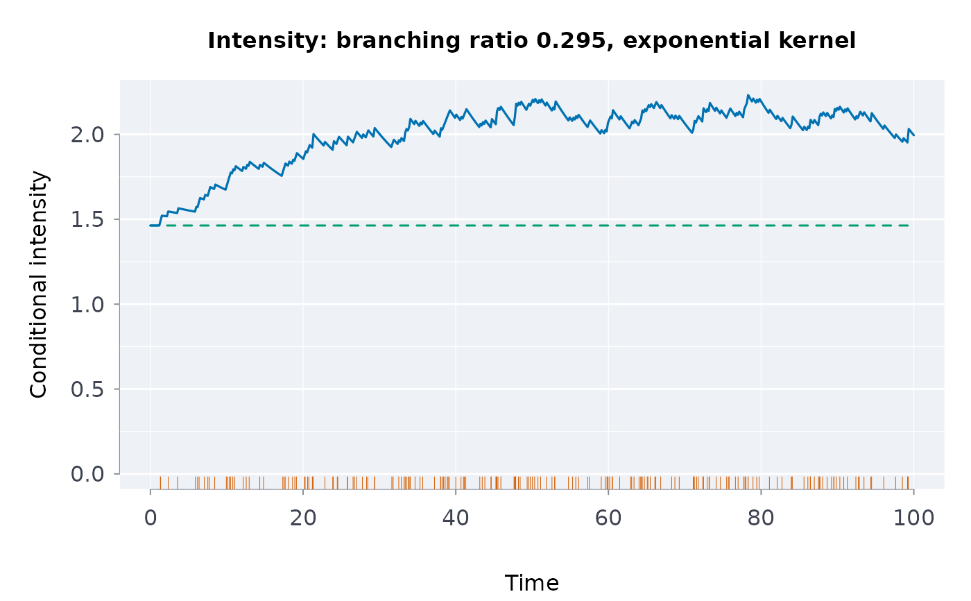
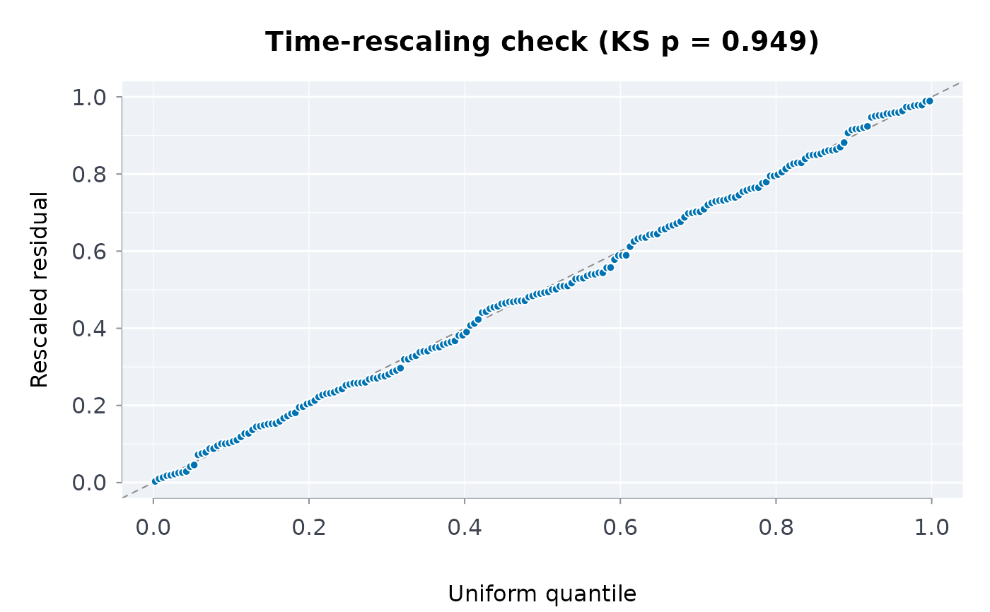
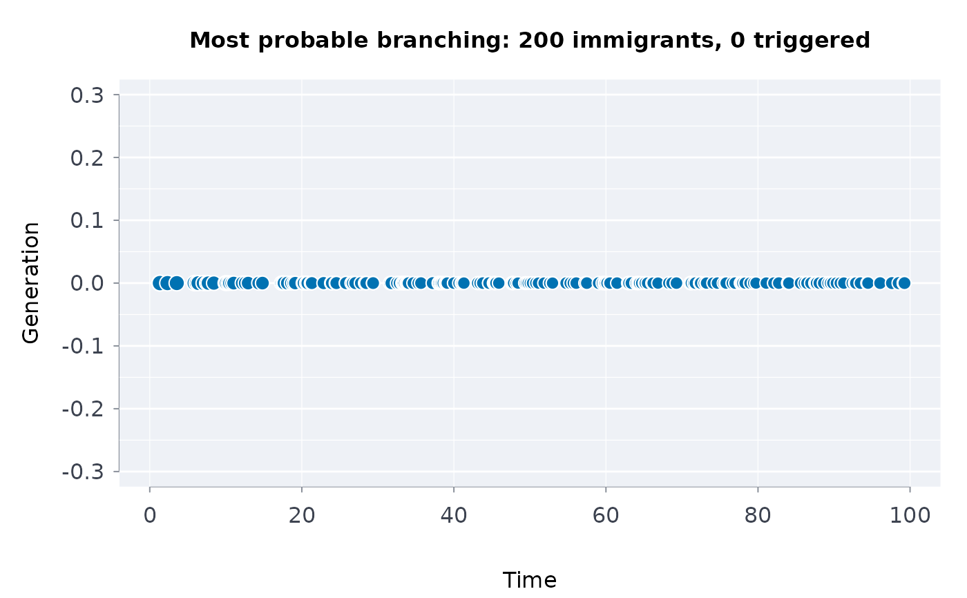
Three views of a chwkfit() result against its events:

"intensity"

the conditional intensity \(\lambda(t) = \nu(t) + \eta \sum_{t_j < t} g(t - t_j)\) over the window, the baseline dashed and the events as ticks along the axis.

"qq"

the time-rescaling residuals of chwkres() against the uniform quantiles: a correct model puts them on the diagonal (the Kolmogorov-Smirnov p-value of the fit in the title).

"tree"

the most probable branching structure: each event drawn at its time and generation, linked to the earlier event (or the baseline) most likely to have triggered it, the probabilities \(\eta g(t_i - t_j)\) and \(\nu(t_i)\) in proportion. At most 5,000 events.

Usage

plothwk(
  fit,
  times,
  what = c("intensity", "qq", "tree"),
  ngrid = 600L,
  ...,
  main = NULL,
  col = NULL,
  pal = NULL
)

Arguments

fit

A chwkfit() result.

times

The event times the fit was made on.

what

One of "intensity", "qq" or "tree".

ngrid

Whole number, default 600: points of the intensity curve.

...

Further arguments to the plot() call that opens the panel.

main, col, pal

The title, colours, and a blpal() name.

Value

The data drawn, invisibly: t and lambda (intensity), uniform and residual (a Q-Q plot), or t, parent (the index of the parent event, 0 for the baseline), prob and generation (tree).

Examples

set.seed(1)
times <- sort(stats::runif(200, 0, 100))
fit <- chwkfit(times, 100)
plothwk(fit, times)

plothwk(fit, times, "qq")

tr <- plothwk(fit, times, "tree")

table(tr$generation)
#> 
#>   0 
#> 200