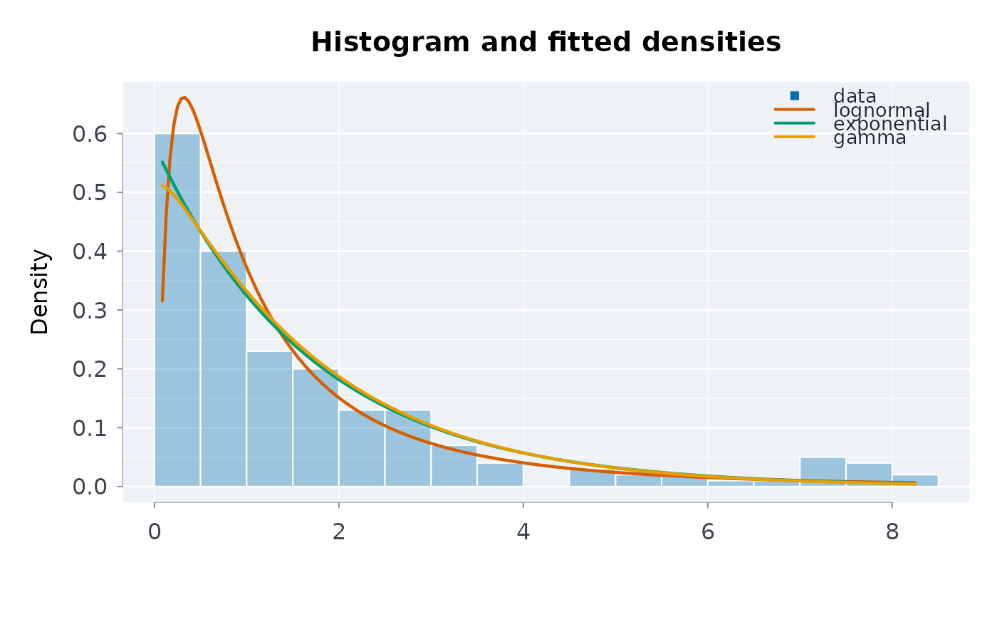
Four views of a dstfit() result: the histogram (or, for counts,
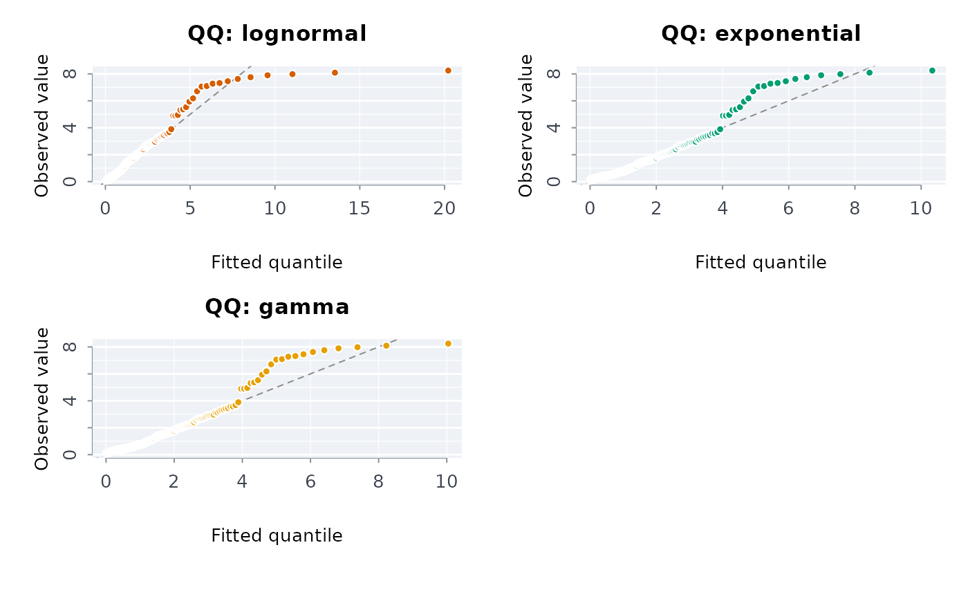
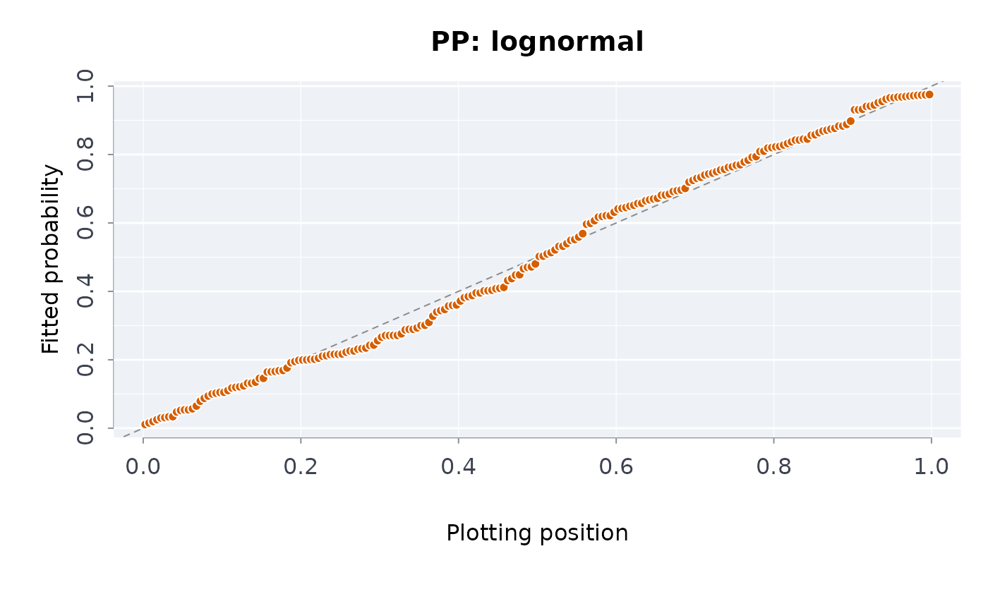
the observed proportions) with each fitted density or mass over it; a QQ plot
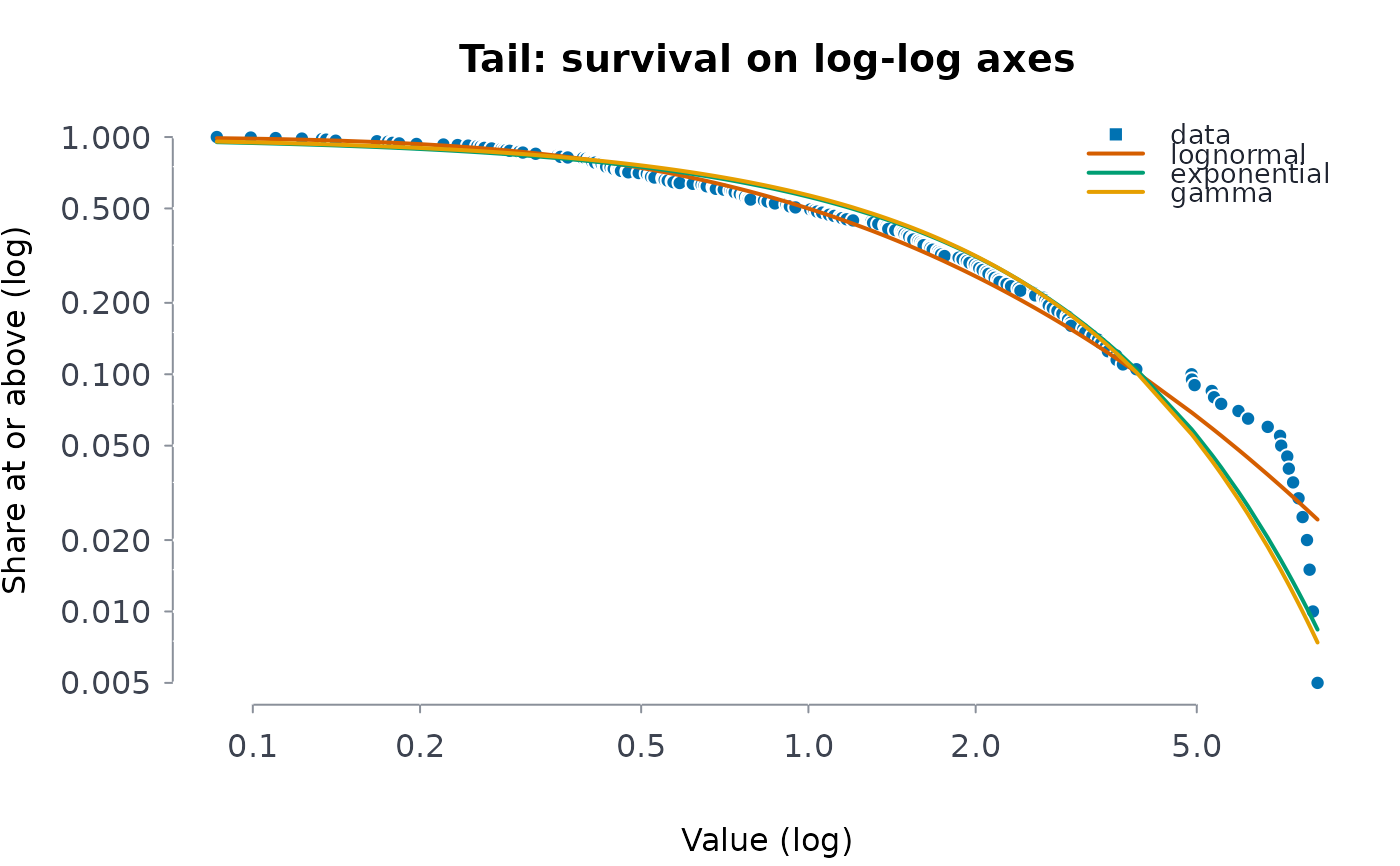
and a PP plot per family; and the empirical survival function on log-log axes
with each fitted survival curve, where a power law is a straight line.
Usage
# S3 method for class 'rmbl_dstfit'
plot(
  x,
  ...,
  which = c("density", "qq", "pp", "tail"),
  fams = NULL,
  main = NULL,
  col = NULL,
  palette = NULL
)
Arguments
- x
A dstfit() result.
- ...
Further graphical arguments to the first panel's plot() call.
- which
One of "density", "qq", "pp" or
"tail".
- fams
Families to draw; default the three best by AIC.
- main, col, palette
The title, colours, and a blpal()
palette name.
Value
The data drawn, invisibly: a data frame with family, x and
y (and for qq and pp the empirical value in y
against the fitted one in x).
Examples
set.seed(2)
f <- dstfit(stats::rlnorm(200), nboot = 0)
plot(f)
 plot(f, which = "qq")
 plot(f, which = "pp", fams = "lognormal")
 plot(f, which = "tail")
 try(plot(f, fams = "beta"))
#> Error : plot: no converged fit for beta
