
Power and minimum detectable effect of a difference-in-differences design
Source:R/panel_causal.R
plnpwr.RdSimulates the design on real untreated data: assigns adoption at random to
units (or clusters) as the study would, adds an effect of known size,
estimates plndid, and counts rejections; so the serial
correlation and the clustering of the real data are carried, as formula-based
power calculations do not.
Usage
plnpwr(
  data,
  unit,
  time,
  y,
  ntrt,
  adopt,
  eff = NULL,
  cl = NULL,
  reps = 200L,
  alpha = 0.05,
  power = 0.8,
  seed = NULL
)
Arguments
- data
A data frame, one row per unit and period.
- unit, time, y
Column names: the unit, the period (numeric, for example a year or a month index) and the outcome.
- ntrt
Units (or clusters) to treat in each replication.
- adopt
Adoption periods to draw from.
- eff
Effect sizes to try (default a grid from 0 to two standard deviations of the outcome).
- cl
Column name of the clusters (default the unit), or two column names for two-way clustering (Cameron, Gelbach and Miller 2011): \(V_a + V_b - V_{ab}\), each term with the small-sample factor of the dimension with fewer clusters, and t on its \(G - 1\) degrees of freedom. A composite cluster (district by month, say) is one column made with
interaction(). Fewer than ten clusters give a warning (CR1 errors are unreliable with so few;wcbis made for that case), and so does a cluster that changes within a unit.- reps
Replications per effect size (default 200).
- alpha
Test level (default 0.05).
- power
For the minimum detectable effect (default 0.8).
- seed
Optional seed for the power simulations.
Value
A data frame of class rmbl_power: effect, power;
attributes mde and size (the rejection rate at effect 0).
Details
In each replication, ntrt units (or clusters, with cl)
are drawn at random and given adoption dates drawn from adopt;
effect is added to their outcomes from adoption on; the cluster-robust
t test of plndid at level alpha is counted as a
rejection. With effect = 0 the rejection rate is the test's actual
size on these data, which should be near alpha: a larger one means the
errors are understated (too few clusters, say), and the power figures are
then optimistic too. The minimum detectable effect is where the power curve
crosses power, by linear interpolation (Burlig, Preonas and Woerman
2020).
References
Burlig F, Preonas L, Woerman M (2020). Panel data and experimental design. Journal of Development Economics 144:102458. doi:10.1016/j.jdeveco.2020.102458
Examples
p <- polex()
pre <- p[p$month <= 12, ]
pw <- plnpwr(pre, "district", "month", "crmrate", ntrt = 10, adopt = 7:10,
eff = c(0, 1, 2, 3), reps = 30, seed = 1)
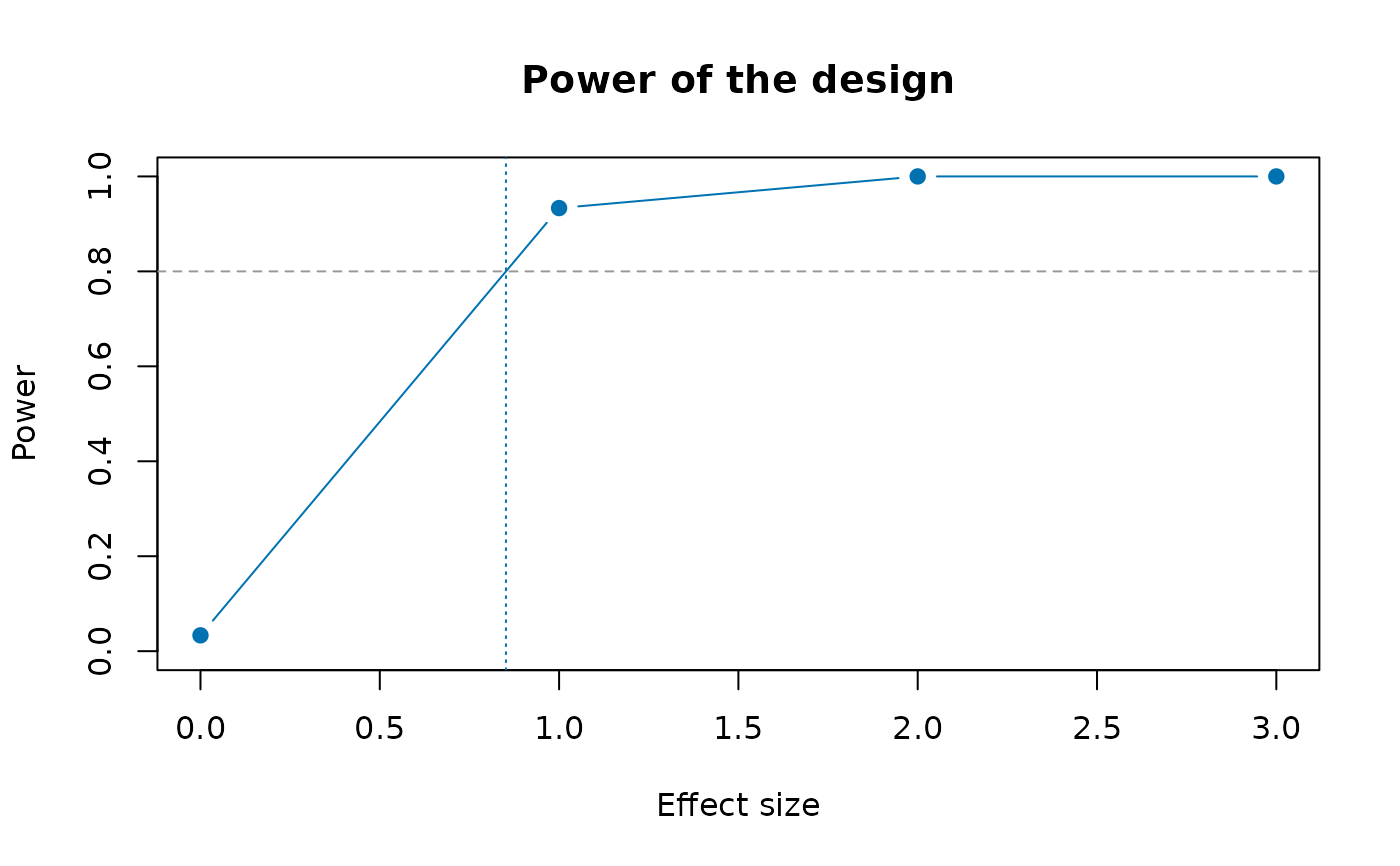
pw
#> ╭── Power of the design ──────────────────────────────────────────────────╮
#> │ Method placebo adoptions on the panel itself │
#> │ Alpha 0.05 │
#> │ Size (no effect) 0.03333 │
#> │ Minimum detectable effect 0.8519 │
#> │ │
#> │ effect power │
#> │ ------ ----- │
#> │ 0 0.033 │
#> │ 1 0.933 │
#> │ 2 1.000 │
#> │ 3 1.000 │
#> │ │
#> │ Power is the share of simulated adoptions, with the effect added, in │
#> │ which the test rejects no effect; the size, at an effect of 0, should │
#> │ be close to alpha. │
#> ╰─────────────────────────────────────────────────────────────────────────╯
plot(pw)
 # your own panel: eight towns over ten years, four adopting a by-law (two
# in 2019, two in 2021), with each town's population, county and income
own <- data.frame(
town = rep(c("A", "B", "C", "D", "E", "F", "G", "H"), each = 10),
year = rep(2015:2024, times = 8)
)
i <- match(own$town, unique(own$town))
own$first <- c(2019, 2019, 2021, 2021, NA, NA, NA, NA)[i]
own$bylaw <- as.integer(!is.na(own$first) & own$year >= own$first)
own$pop <- c(12, 30, 8, 22, 15, 40, 9, 18)[i] * 1000
own$county <- rep(c("North", "South"), 4)[i]
own$income <- 50 + own$year - 2015 + cos(seq_len(80))
own$rate <- 30 + i + 0.5 * (own$year - 2015) - 4 * own$bylaw +
0.2 * own$income + sin(seq_len(80))
# the power of four towns adopting in 2017 or 2018, from the years before
# any by-law
plnpwr(own[own$year <= 2018, ], "town", "year", "rate", ntrt = 4,
adopt = 2017:2018, eff = c(0, 2, 4), reps = 20, seed = 1)
#> ╭── Power of the design ──────────────────────────────────────────────────╮
#> │ Method placebo adoptions on the panel itself │
#> │ Alpha 0.05 │
#> │ Size (no effect) 0 │
#> │ Minimum detectable effect 3.333 │
#> │ │
#> │ effect power │
#> │ ------ ----- │
#> │ 0 0.000 │
#> │ 2 0.400 │
#> │ 4 1.000 │
#> │ │
#> │ Power is the share of simulated adoptions, with the effect added, in │
#> │ which the test rejects no effect; the size, at an effect of 0, should │
#> │ be close to alpha. │
#> ╰─────────────────────────────────────────────────────────────────────────╯