
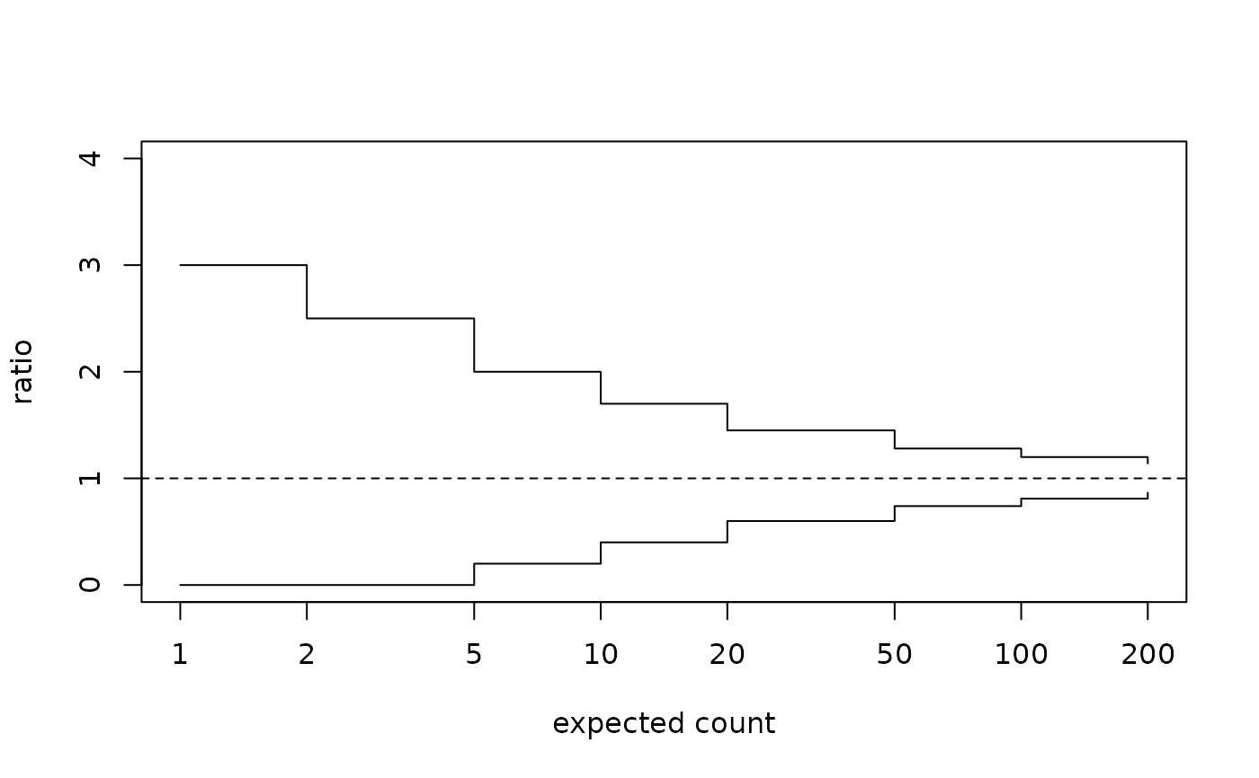
Gives the range within which an area's ratio of observed to expected would fall, for a given expected count, if the area were no different from the overall experience. Plotted against the expected count these limits form a funnel: wide for small areas, narrow for large ones. A funnel plot is the alternative to a league table: it shows directly that a small area's ratio can wander far from one without meaning anything.
Usage
fnllim(expd, target = 1, lvls = c(0.95, 0.998))Arguments
- expd
Numeric vector of expected counts (positive) at which to compute limits, for example a grid from the smallest to the largest area.
- target
Number, default
1: the ratio the limits are centred on. One is the overall experience.- lvls
Numeric vector of two-sided coverage levels in (0, 1), default
c(0.95, 0.998); one pair of limits per level.
Value
A data frame with one row per expected count and level, sorted by
level then expected count, with numeric columns expected,
level, lower and upper (the limits on the ratio
scale).
Details
For expected count \(E\), target ratio \(\rho\) and coverage \(1 - a\), the limits are $$\frac{Q(a/2;\ \rho E)}{E},\quad \frac{Q(1 - a/2;\ \rho E)}{E}$$ with \(Q\) the Poisson quantile function. They are exact Poisson quantiles divided by the expected count, so they are the discrete counterpart of the usual normal funnel and stay correct at the small expected counts where the normal version goes below zero. Because the Poisson is discrete the limits move in steps of \(1/E\). The usual pair of levels, 0.95 and 0.998, corresponds to about two and three standard deviations.
Errors: non-positive, infinite or missing expected counts (missing
values are dropped); a non-positive target; a level outside
(0, 1).
References
Spiegelhalter, D. J. (2005). Funnel plots for comparing institutional performance. Statistics in Medicine 24(8), 1185-1202. doi:10.1002/sim.1970
Advanced Statistics in Criminology and Criminal Justice discusses the funnel plot as the display of the relationship between an estimate and the sample size behind it.
Lawson, A. B. Using R for Bayesian Spatial and Spatio-Temporal Health Modeling. Chapman and Hall/CRC, on the Poisson counts these limits are built from.
Examples
# The funnel narrows as the expected count grows, which is the whole
# point: a ratio of 2 means nothing at an expected count of 2 and a
# great deal at an expected count of 200.
fnllim(c(2, 20, 200))
#> expected level lower upper
#> 1 2 0.950 0.000 2.500
#> 2 20 0.950 0.600 1.450
#> 3 200 0.950 0.865 1.140
#> 4 2 0.998 0.000 4.000
#> 5 20 0.998 0.400 1.750
#> 6 200 0.998 0.790 1.225
# one 90 percent funnel around a target ratio of 1.2
fnllim(c(5, 50), target = 1.2, lvls = 0.90)
#> expected level lower upper
#> 1 5 0.9 0.40 2.00
#> 2 50 0.9 0.96 1.46
# a funnel drawn with base graphics
e <- c(1, 2, 5, 10, 20, 50, 100, 200)
f <- fnllim(e, lvls = 0.95)
plot(f$expected, f$upper, type = "s", log = "x", ylim = c(0, 4),
xlab = "expected count", ylab = "ratio")
lines(f$expected, f$lower, type = "s")
abline(h = 1, lty = 2)
 try(fnllim(10, lvls = 1))
#> Error : `lvls` must lie strictly inside (0, 1)