A dose-response across generations of exposure

For counts of an outcome (suicidal thoughts, distress) among people with 0, 1 or 2 generations of residential school attendance in their family (or any ordered exposure), the odds ratio of each level against the lowest level, with Woolf intervals, and the Cochran-Armitage test for a trend across the levels.

Usage

exptrnd(cases, n, dose = seq_along(cases) - 1L, conflvl = 0.95)

Arguments

cases

Number with the outcome at each exposure level.

n

Number of people at each level.

dose

The exposure levels, in order (default 0, 1, 2, ...); the trend test scores them.

conflvl

Confidence level of the odds ratios' intervals (default 0.95).

Value

A data frame with dose, cases, n, proportion, orratio, lower, upper; the trend test is the attribute trend (an htest).

Details

With \(a_k\) cases and \(b_k = n_k - a_k\) non-cases at level \(k\), the odds ratio against the lowest level is \((a_k/b_k)/(a_1/b_1)\), with Woolf's interval \(\exp\{\log OR \pm z\sqrt{1/a_k + 1/b_k + 1/a_1 + 1/b_1}\}\). When any cell is empty, one half is added to every cell of every level (Haldane-Anscombe), so every odds ratio is finite. The trend test is the Cochran-Armitage test (prop.trend.test) with the levels as scores. Counts must be unweighted. For a complex survey, take the weighted analysis from the survey itself (svydes): this function is for published or aggregated counts.

References

McQuaid RJ, et al. (2017), see genexpo.

Examples

# made-up counts by 0, 1 and 2 generations of attendance, to show the
# computation
et <- exptrnd(cases = c(60, 95, 70), n = c(500, 520, 300))
et
#> ╭── Odds by level of exposure, with the trend ────────────────────────────────╮
#> │   Levels  3                                                                 │
#> │   People  1,320                                                             │
#> │   Cases   225                                                               │
#> │   Trend   chi-square 17.86 on 1 df, p < 0.001                               │
#> │                                                                             │
#> │   dose  cases    n  proportion  orratio  interval                           │
#> │   ----  -----  ---  ----------  -------  ------------                       │
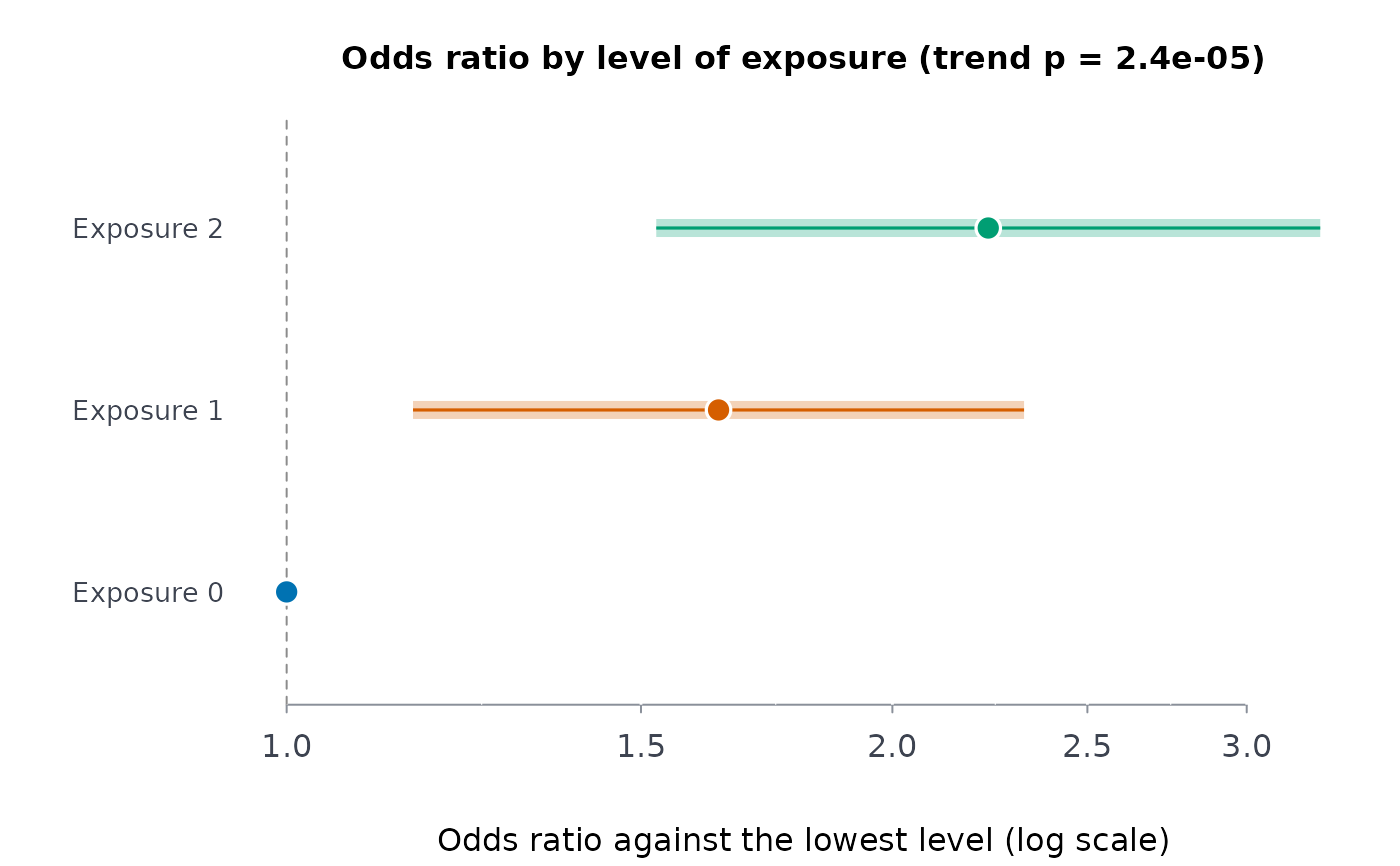
#> │      0     60  500      0.1200    1.000  [1.00, 1.00]                       │
#> │      1     95  520      0.1827    1.639  [1.16, 2.33]                       │
#> │      2     70  300      0.2333    2.232  [1.53, 3.26]                       │
#> │                                                                             │
#> │   At the highest level (2) the odds of a case are 2.232 [1.526, 3.263]      │
#> │   times those at the lowest (0).                                            │
#> │   The odds rise with exposure: the trend test rejects a flat trend (p <     │
#> │   0.001, below 0.05).                                                       │
#> │                                                                             │
#> │   orratio: the odds of a case at each level over the odds at the lowest     │
#> │   (Woolf's interval); the trend test asks whether they rise with level.     │
#> ╰─────────────────────────────────────────────────────────────────────────────╯
plot(et)