
An event study: the effect period by period around adoption
Source:R/policy_evaluation.R
evstudy.RdLeads and lags of a policy's adoption, from a two-way fixed-effects regression on indicators of the time since adoption, with a joint test that the leads are zero (no effect before the policy, the testable part of parallel trends).
Usage
evstudy(
  data,
  unit,
  time,
  y,
  ftreat,
  leads = 4L,
  lags = 4L,
  ref = -1L,
  bin = TRUE,
  covs = NULL,
  cl = NULL,
  conflvl = 0.95,
  w = NULL
)
Arguments
- data
A data frame, one row per unit and period.
- unit, time, y
Column names: the unit, the period (numeric, for example a year or a month index) and the outcome.
- ftreat
Column name of the period a unit is first treated (
NA, 0 orInffor a unit never treated). Treatment is taken as staying on.- leads, lags
The number of periods before and after adoption to estimate (default 4 and 4).
- ref
The period left out (default -1).
- bin
Bin the periods beyond the window into its end points (default
TRUE).- covs
Optional column names of time-varying controls.
- cl
Column name of the clusters (default the unit), or two column names for two-way clustering (Cameron, Gelbach and Miller 2011): \(V_a + V_b - V_{ab}\), each term with the small-sample factor of the dimension with fewer clusters, and t on its \(G - 1\) degrees of freedom. A composite cluster (district by month, say) is one column made with
interaction(). Fewer than ten clusters give a warning (CR1 errors are unreliable with so few;wcbis made for that case), and so does a cluster that changes within a unit.- conflvl
Confidence level of the intervals reported (default 0.95).
- w
Optional column name of non-negative weights, such as population or matching weights, for weighted least squares with weighted within-means. Rows of weight 0 take no part in the fit.
Value
A data frame of class rmbl_event_study: evtm,
estimate, se, lower, upper, t,
p_value, with the reference period as a row of zeros; attributes
pretrend (a list: F, df1, df2, p_value),
vcov (of the estimated event times), n, clusters,
conflvl. plot() draws it.
Details
With \(G_i\) the first treated period of unit \(i\) and \(k =
t - G_i\), $$Y_{it} = \sum_{k = -L, k \ne r}^{M} \gamma_k \mathbf 1(t -
G_i = k) + X_{it}'\theta + \delta_i + \mu_t + \varepsilon_{it},$$ with the reference period
\(r\) (default -1, the period before adoption) left out. Times beyond the
window are binned into its end points (bin = TRUE), or dropped. Units
never treated have every indicator 0. The variance and degrees of freedom are
those of plndid. The pre-trend test is the Wald statistic
\(W = \hat\gamma_{pre}'\hat V_{pre}^{-1}\hat\gamma_{pre}\), reported as
\(F = W/q\) on \(q\) and \(G - 1\) degrees of freedom.
With staggered adoption and effects that change over time, the lead and lag
coefficients can mix in effects from other periods (Sun and Abraham 2021);
stgatt gives the event-time effects free of that.
References
Sun L, Abraham S (2021). Estimating dynamic treatment effects in
event studies with heterogeneous treatment effects. Journal of Econometrics
225(2):175-199.
doi:10.1016/j.jeconom.2020.09.006
Applied to the effect of donations on police stops, block by quarter: Zorro Medina A, Hackett D, Green D, Vargas R (2025). Evidence of donor bias in Chicago police stops. arXiv:2504.15140 (https://arxiv.org/abs/2504.15140).
Examples
p <- polex()
es <- evstudy(p, "district", "month", "crmrate", "refmonth", leads = 3,
lags = 4)
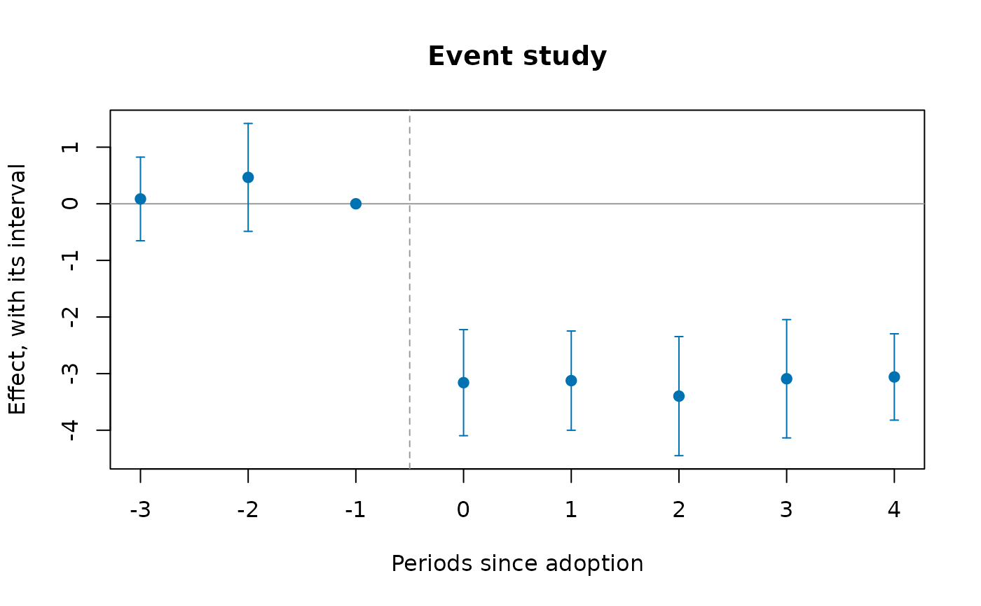
es
#> ╭── Event study ──────────────────────────────────────────────────────────────╮
#> │ Method fixed-effects regression on the periods since │
#> │ adoption │
#> │ Observations 720 │
#> │ Clusters 20 │
#> │ Periods -3 to 4 since adoption │
#> │ Reference period -1 │
#> │ Confidence 95% │
#> │ Leads jointly zero F(2, 19) = 1.016, p = 0.381 │
#> │ │
#> │ evtm estimate se 95% CI t p_value │
#> │ ---- -------- ------ ---------------- ------ ------- │
#> │ -3 0.086 0.3530 [-0.653, 0.824] 0.243 0.811 │
#> │ -2 0.466 0.4552 [-0.487, 1.419] 1.024 0.319 │
#> │ -1 0.000 0.0000 [0.000, 0.000] │
#> │ 0 -3.160 0.4476 [-4.097, -2.223] -7.059 < 0.001 │
#> │ 1 -3.124 0.4189 [-4.001, -2.247] -7.458 < 0.001 │
#> │ 2 -3.398 0.5025 [-4.450, -2.346] -6.761 < 0.001 │
#> │ 3 -3.091 0.4993 [-4.136, -2.046] -6.191 < 0.001 │
#> │ 4 -3.059 0.3644 [-3.822, -2.296] -8.394 < 0.001 │
#> │ │
#> │ Each row is the effect that many periods from adoption, measured │
#> │ against the reference period. The leads are jointly consistent with │
#> │ zero, the testable part of parallel trends. │
#> ╰─────────────────────────────────────────────────────────────────────────────╯
attr(es, "pretrend")$p_value
#> [1] 0.380962
plot(es)
 # your own panel: eight towns over ten years, four adopting a by-law (two
# in 2019, two in 2021), with each town's population, county and income
own <- data.frame(
town = rep(c("A", "B", "C", "D", "E", "F", "G", "H"), each = 10),
year = rep(2015:2024, times = 8)
)
i <- match(own$town, unique(own$town))
own$first <- c(2019, 2019, 2021, 2021, NA, NA, NA, NA)[i]
own$bylaw <- as.integer(!is.na(own$first) & own$year >= own$first)
own$pop <- c(12, 30, 8, 22, 15, 40, 9, 18)[i] * 1000
own$county <- rep(c("North", "South"), 4)[i]
own$income <- 50 + own$year - 2015 + cos(seq_len(80))
own$rate <- 30 + i + 0.5 * (own$year - 2015) - 4 * own$bylaw +
0.2 * own$income + sin(seq_len(80))
# three years either side of adoption, weighted by population
evstudy(own, "town", "year", "rate", "first", leads = 3, lags = 3,
w = "pop")
#> ╭── Event study ──────────────────────────────────────────────────────────────╮
#> │ Method fixed-effects regression on the periods since │
#> │ adoption │
#> │ Observations 80 │
#> │ Clusters 8 │
#> │ Periods -3 to 3 since adoption │
#> │ Reference period -1 │
#> │ Confidence 95% │
#> │ Leads jointly zero F(2, 7) = 0.044, p = 0.957 │
#> │ │
#> │ evtm estimate se 95% CI t p_value │
#> │ ---- -------- ------ ---------------- ------- ------- │
#> │ -3 -0.327 1.1159 [-2.965, 2.312] -0.293 0.778 │
#> │ -2 -0.098 0.4011 [-1.046, 0.851] -0.244 0.814 │
#> │ -1 0.000 0.0000 [0.000, 0.000] │
#> │ 0 -4.076 0.2689 [-4.712, -3.440] -15.158 < 0.001 │
#> │ 1 -4.214 0.8271 [-6.170, -2.258] -5.095 0.001 │
#> │ 2 -4.368 1.3432 [-7.544, -1.192] -3.252 0.014 │
#> │ 3 -3.964 0.8082 [-5.875, -2.053] -4.904 0.002 │
#> │ │
#> │ Each row is the effect that many periods from adoption, measured │
#> │ against the reference period. The leads are jointly consistent with │
#> │ zero, the testable part of parallel trends. │
#> ╰─────────────────────────────────────────────────────────────────────────────╯