
Search and rescue: detection, coverage and the best use of effort
Source:vignettes/search-and-rescue.Rmd
search-and-rescue.RmdSearch theory began with Koopman’s work for the U.S. Navy (1946) and
is how search and rescue services plan a search: how likely a sensor is
to see the object at a given distance, how much ground a search covers,
how likely the object is to be in each area, and where a limited effort
does the most good. Frost’s The Theory of Search: A Simplified
Explanation (1996) explains it for search planners in four chapters
of figures. This vignette walks those chapters and draws every one of
the book’s 36 figures with srchfig(), which builds each
from the package’s functions with the book’s parameters.
srchfig() with no argument lists them and says how each is
drawn: from the model, as a schematic, or as an approximation where the
book’s plate cannot be recovered exactly.
The functions behind the figures work on any inputs:
ltrlrng() (lateral range curves), swpwdth()
(sweep width), srchpod() and pswppod()
(probability of detection), srchscs() (probability of
success and the update after a search), datumpmap() (where
the object may be), opteffort(), optcrcsrch()
and optsqr() (the best use of effort). The book’s figures
come first; Your own search then runs
each function on numbers of your own.
Datums and probability maps
Figure 3-1. A point datum is a circular normal
distribution of possible positions. The probability that the object is
within R standard deviations of the datum is
POC = 1 - exp(-R^2 / 2).
srchfig("3-1")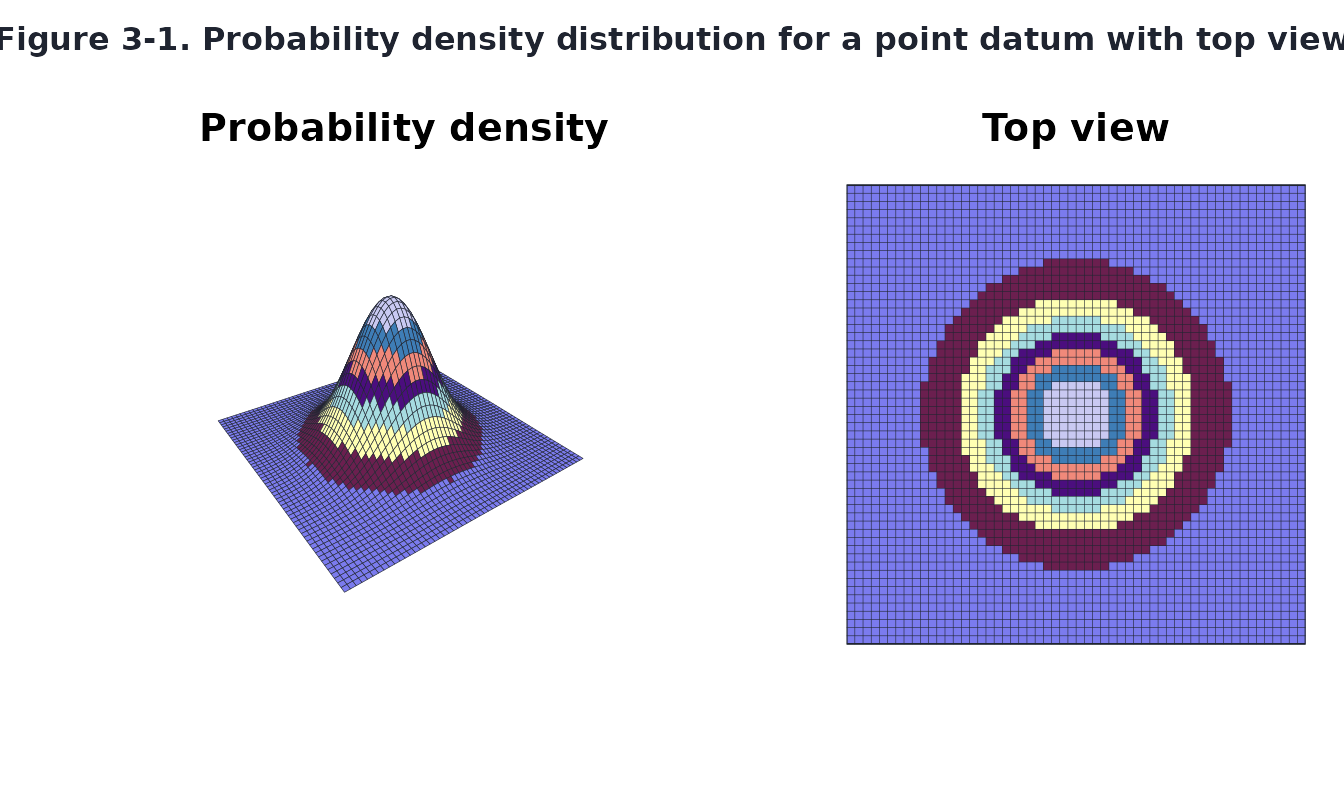
Figures 3-2, 3-3 and 3-5. The square circumscribed
about a circle of radius R holds
(2 Phi(R) - 1)^2 of the distribution: 47% for one standard
deviation, 58% for the total probable error of position
E = sqrt(2 ln 2) = 1.1774 standard deviations (the radius
holding 50%), and 65% for the simplified method’s first search radius of
1.1 E.
srchfig("3-2")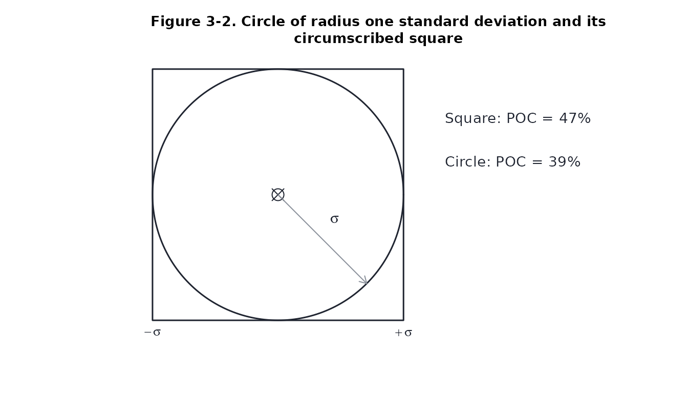
srchfig("3-3")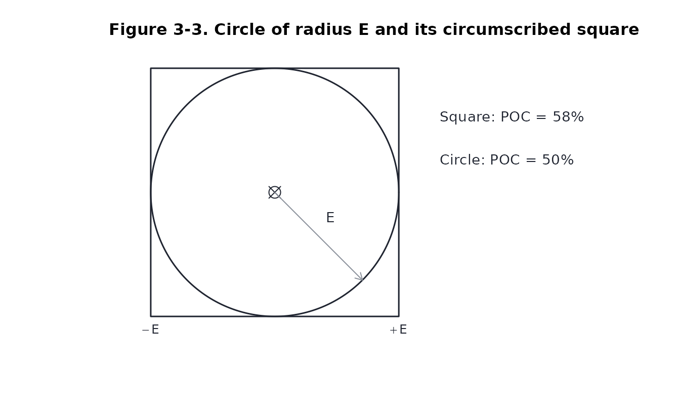
srchfig("3-5")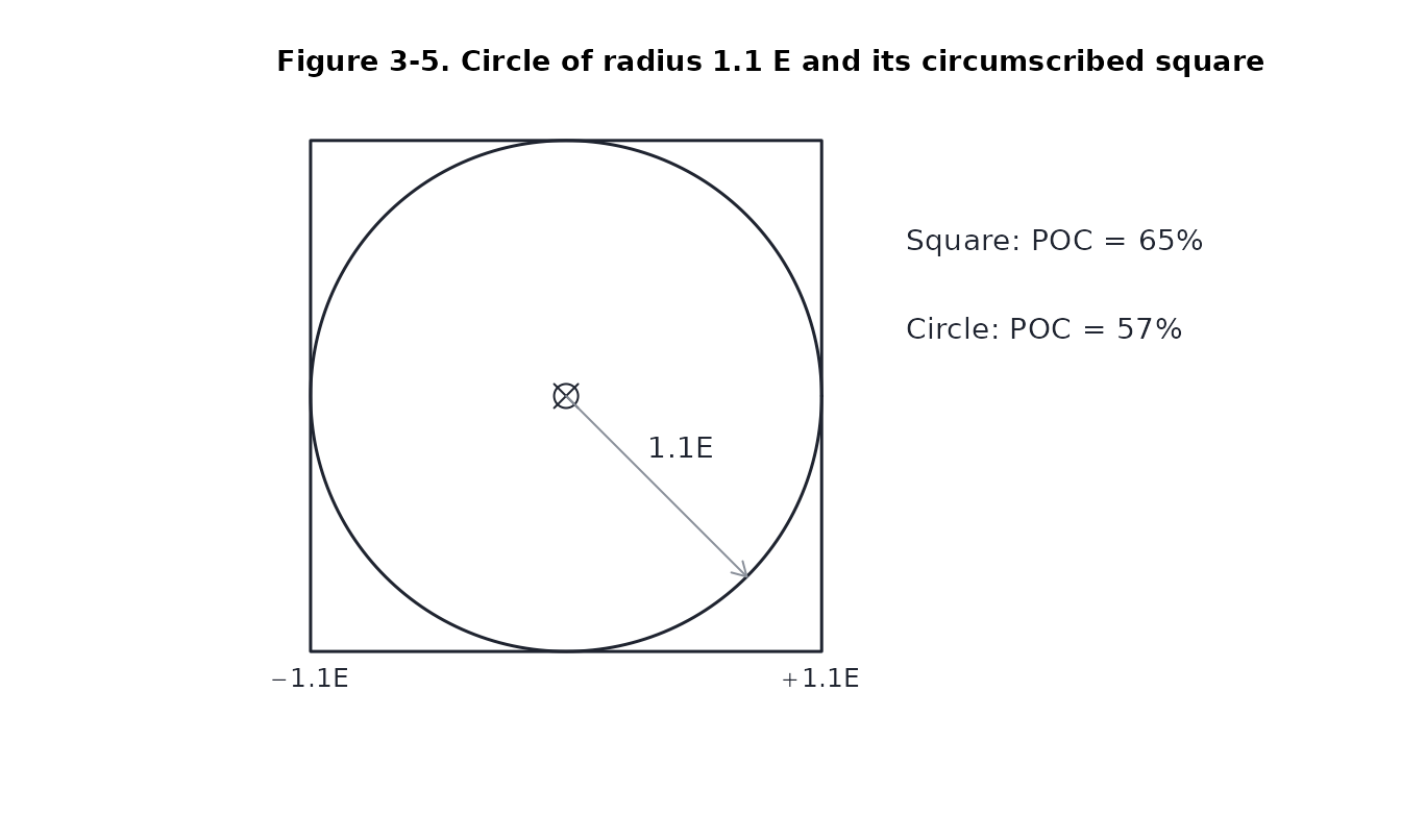
Figure 3-4. A probability map lays a grid over the
distribution. With cells 2E wide the centre holds 57.91%, a
side cell 9.08% and a corner 1.42%.
srchfig("3-4")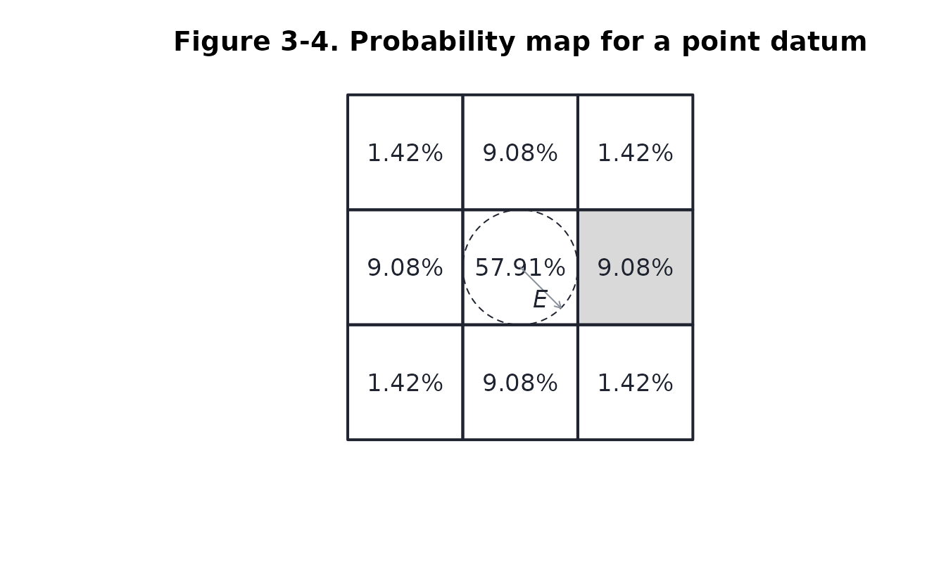
Figures 3-6 and 3-7. The simplified method extended
a point datum to a line by drawing circles at the two end points and
boxing them in. The density this implies is drawn as a circular normal
spread along the segment (datum = "line"), an approximation
of the book’s plate.
srchfig("3-6")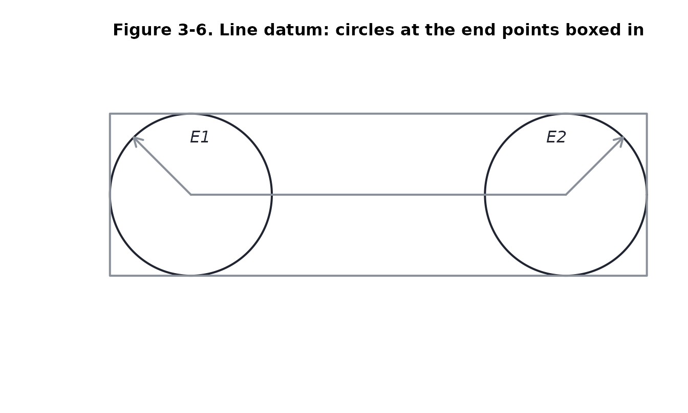
srchfig("3-7")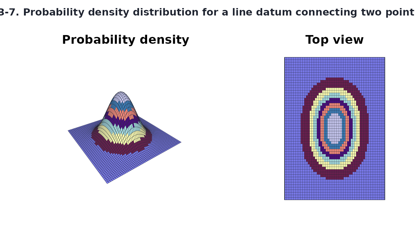
Figures 3-8 to 3-10. A simpler line datum is normal
across the line and uniform along it, with nothing beyond its ends
(datum = "corridor"). A strip one standard deviation either
side holds 68%, a strip of 2E holds 76.1%, and dividing
strips into cells along the line gives the completed map of figure
3-10.
srchfig("3-8")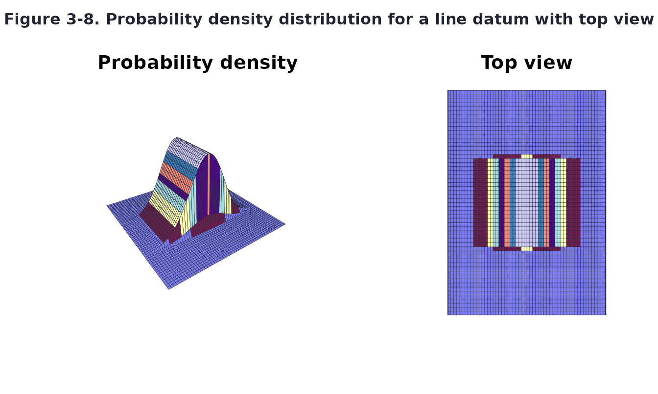
srchfig("3-9")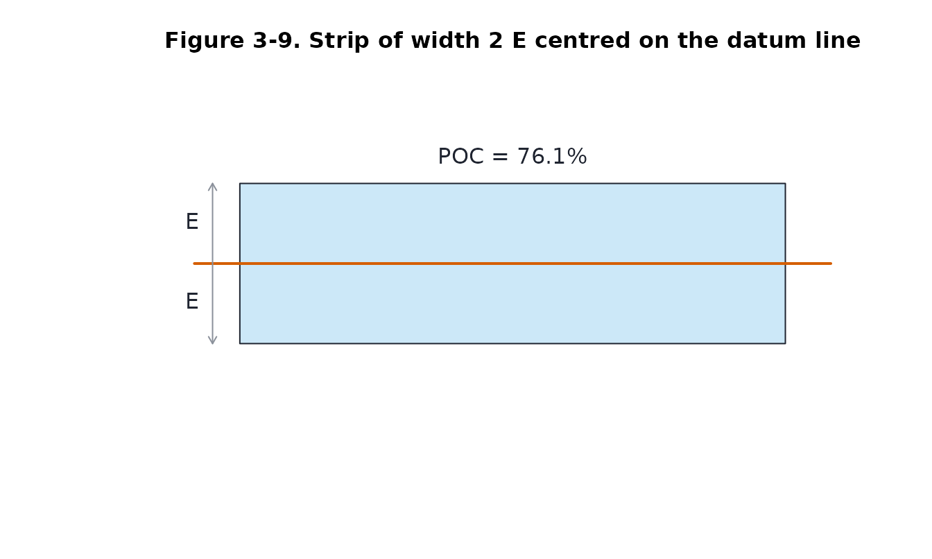
srchfig("3-10")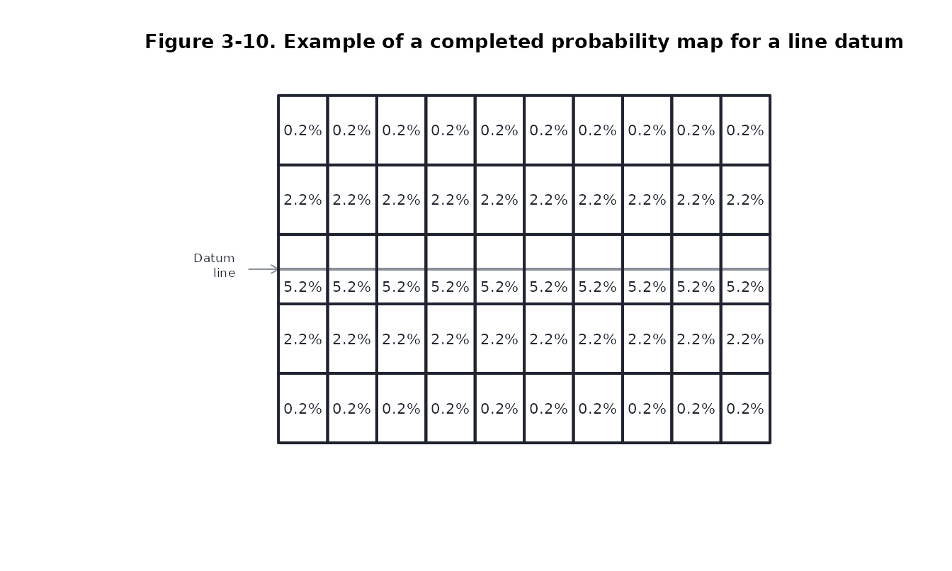
Figures 3-11 and 3-12. An area datum spreads the probability evenly: each of 20 equal cells holds 5%.
srchfig("3-11")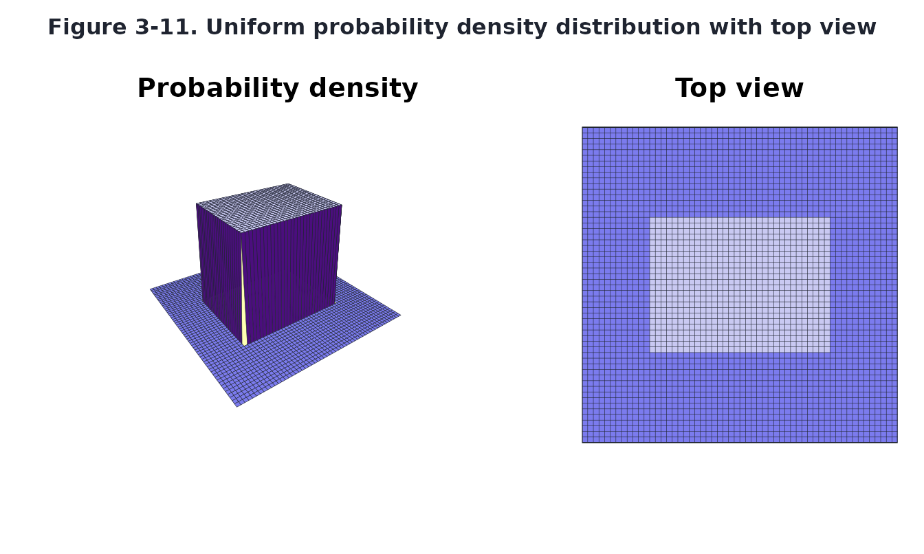
srchfig("3-12")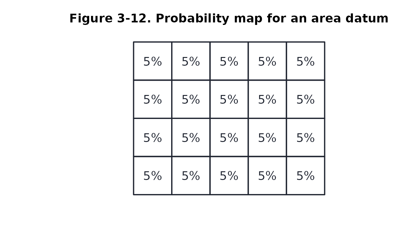
Figures 3-13 and 3-14. A generalized datum takes the
planner’s own cell probabilities (datum = "general",
wts =). The book’s surface is illustrative; here it is
drawn from the cells of figure 3-14.
srchfig("3-13")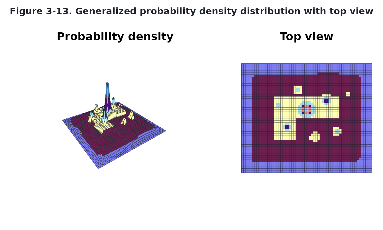
srchfig("3-14")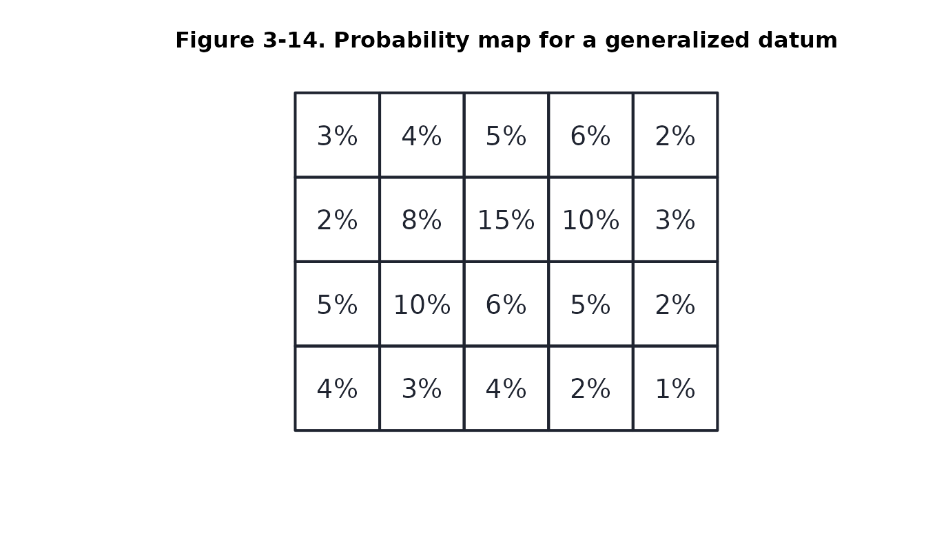
Lateral range curves and sweep width
Figure 4-1. A lateral range curve p(x)
is the probability of detecting an object that passes at distance
x from the track. The sweep width is its area,
W = integral of p(x) dx; the dashed rectangles have the
same area.
srchfig("4-1")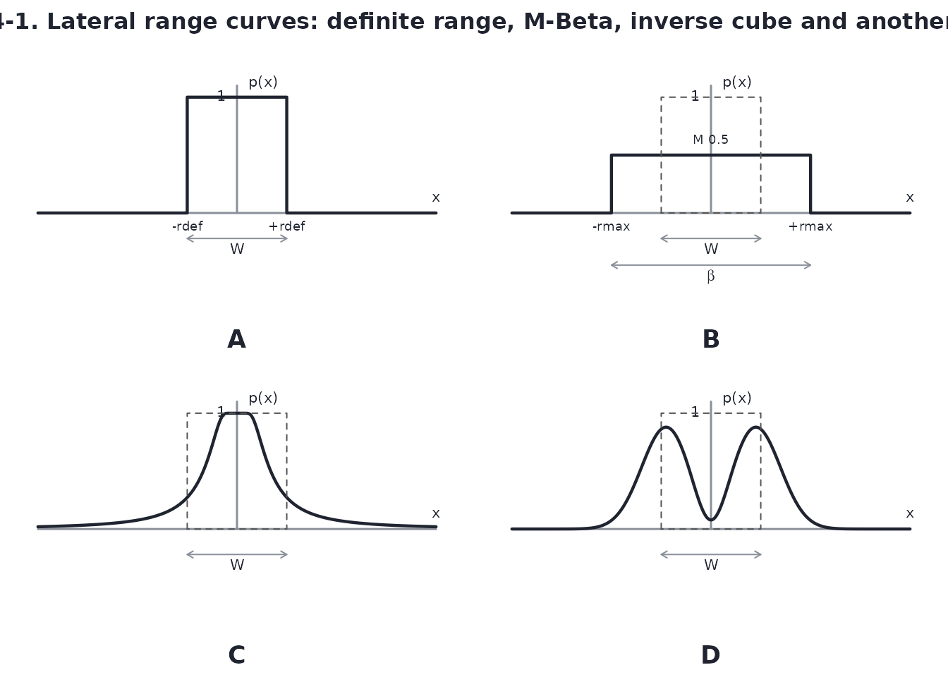
Figures 4-2 and 4-3. A definite range sensor sees
everything within W / 2 of its track and nothing beyond: it
sweeps a strip exactly W wide.
srchfig("4-2")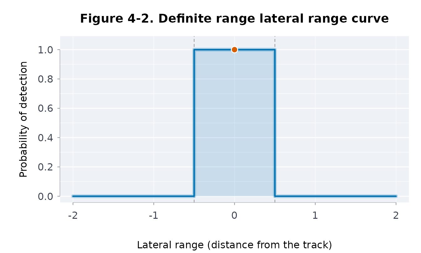
srchfig("4-3")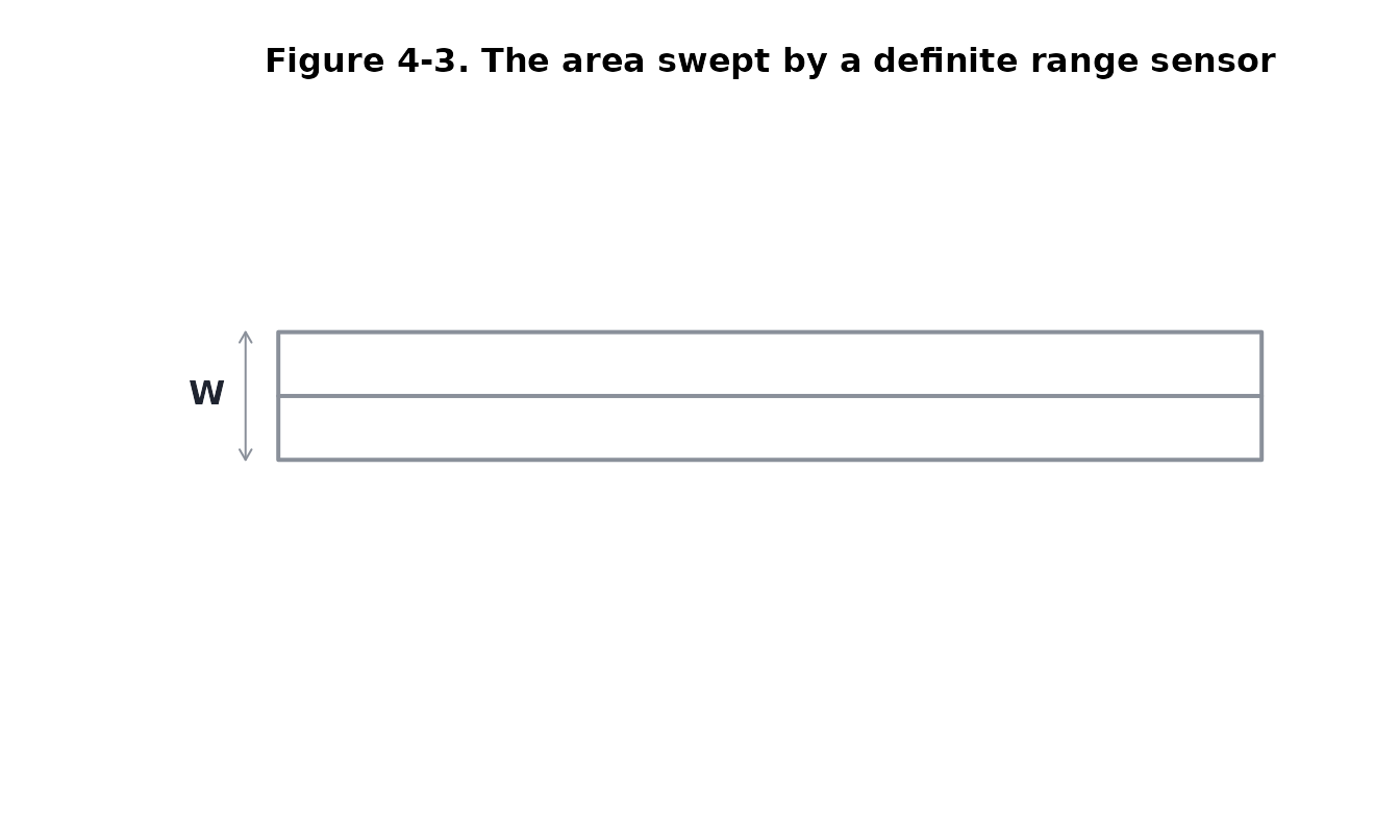
Figures 4-4 and 4-5. The M-Beta curve has height
M over a width of W / M; with
M = 0.5 and M = 0.25 the sweep width is
unchanged.
srchfig("4-4")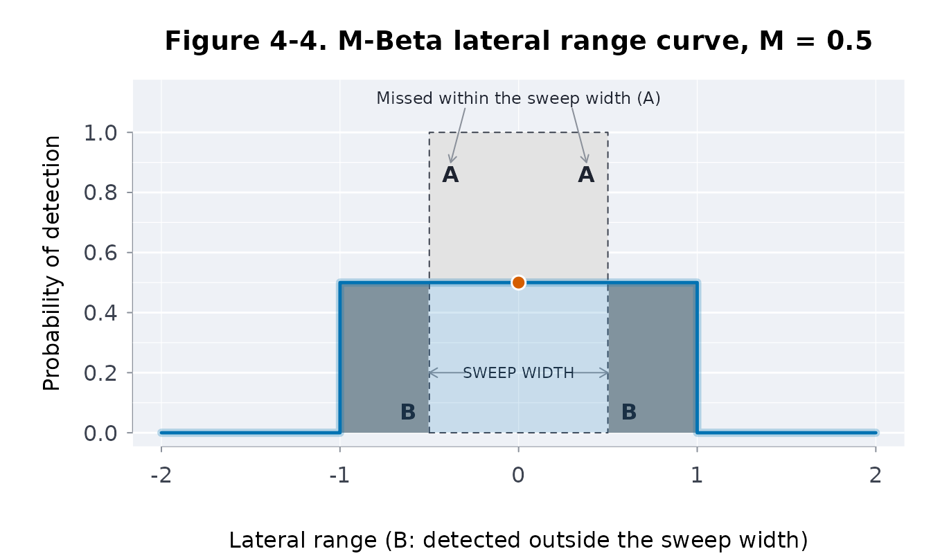
srchfig("4-5")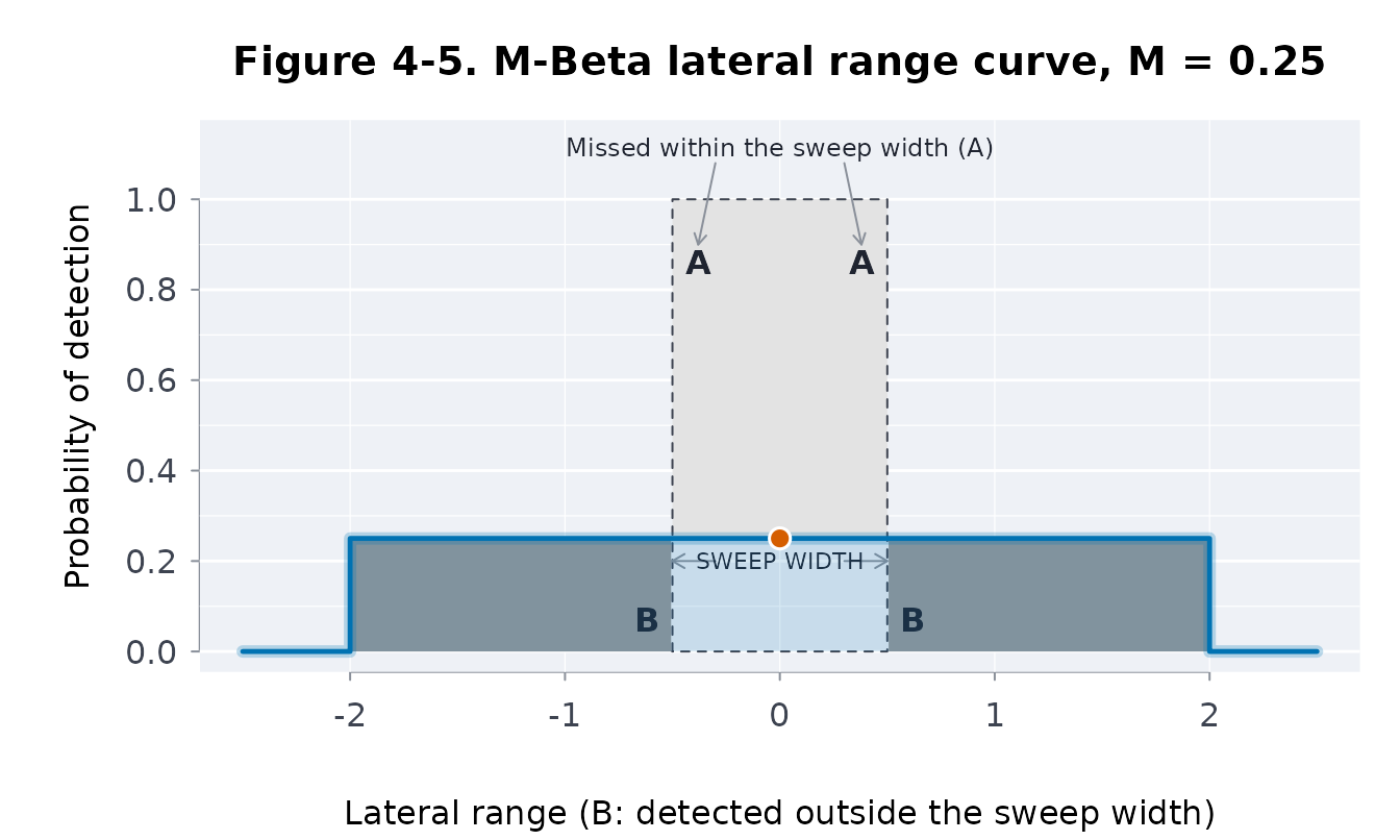
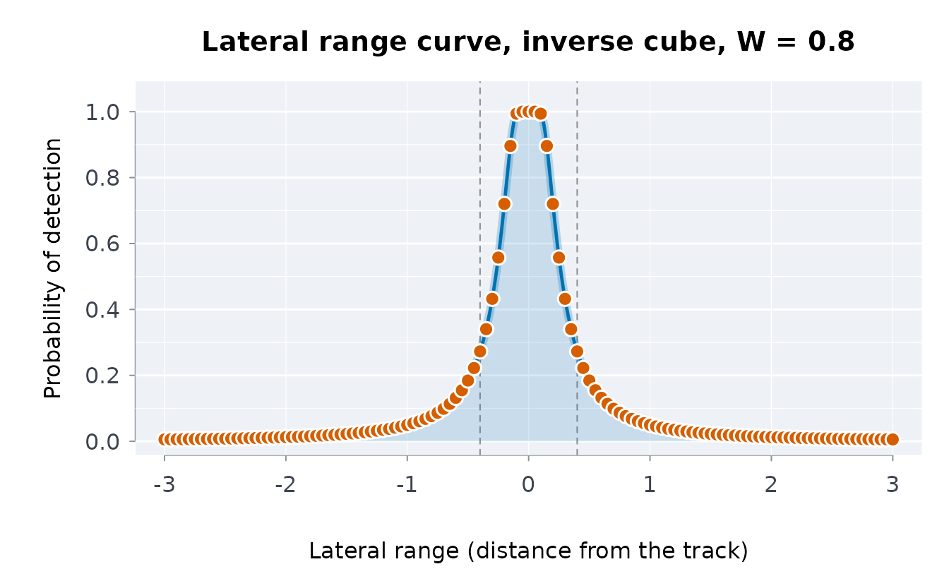
Figures 4-6 and 4-7. Koopman’s inverse cube law
takes the chance of a glimpse to be proportional to the solid angle of
the wake, k h / r^3, which gives
p(x) = 1 - exp(-W^2 / (4 pi x^2)). Its sweep width is
W: the objects missed inside the sweep width (A) balance
those seen outside it (B).
srchfig("4-6")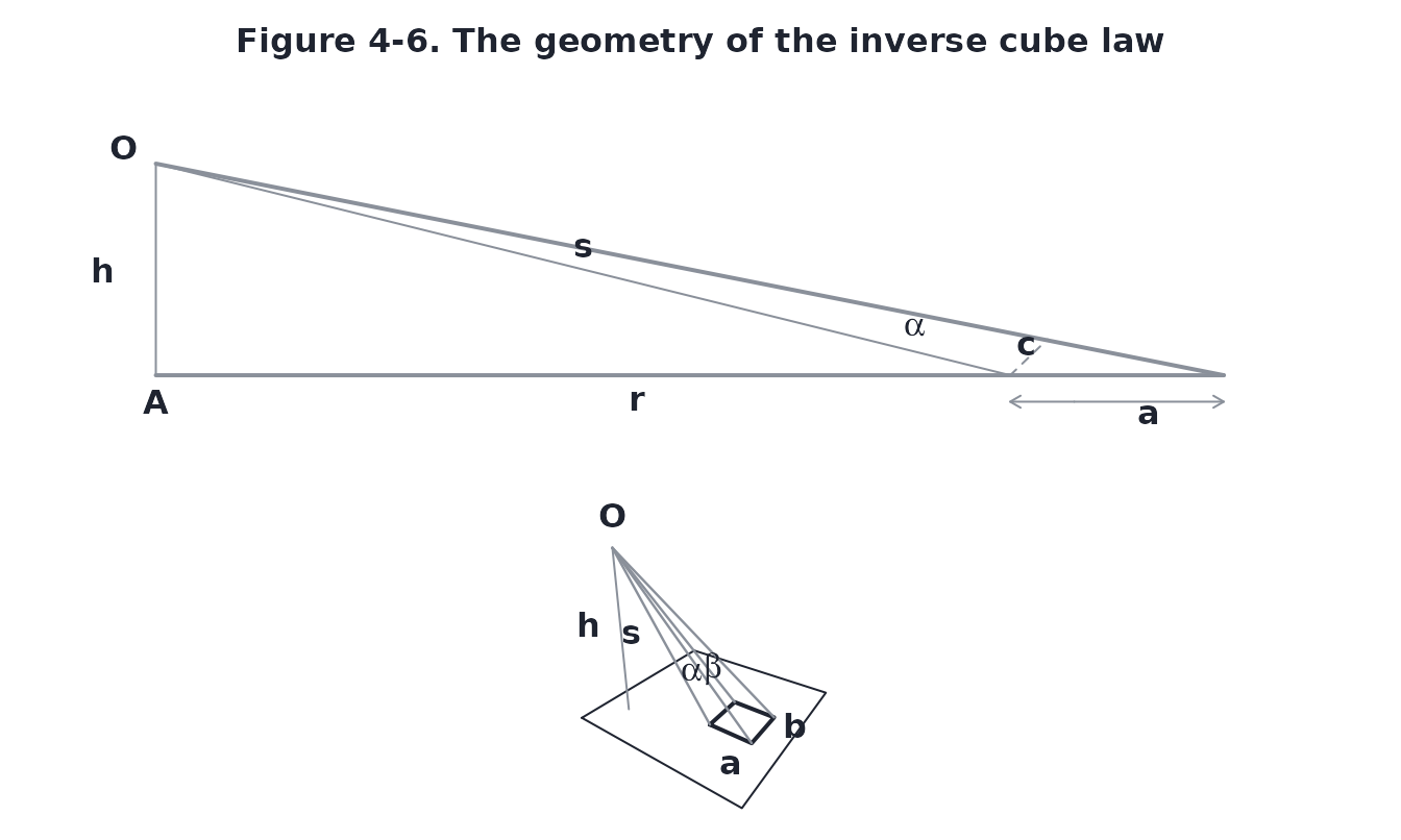
srchfig("4-7")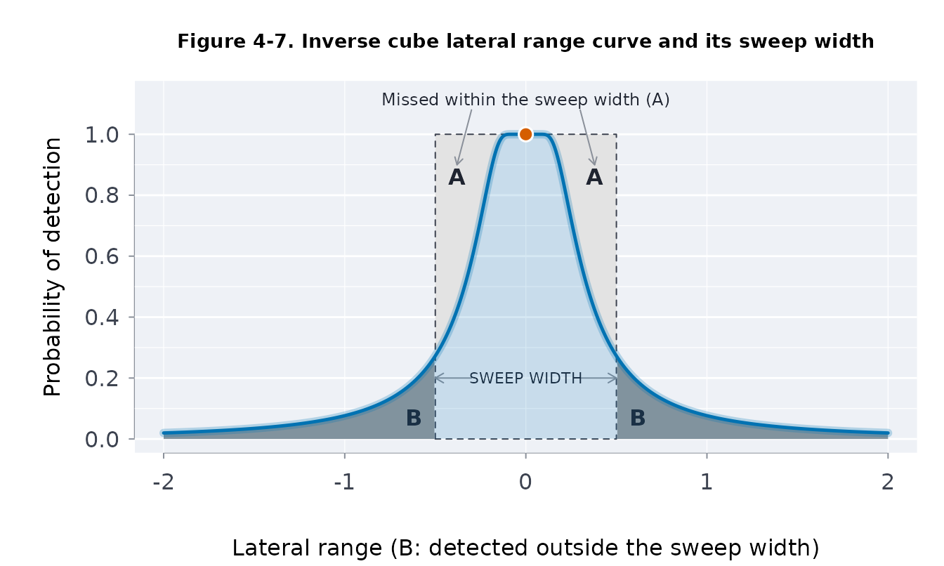
Effort, coverage and probability of detection
Figure 5-1. Search effort is sweep width times track
length, Z = W L, and coverage is effort over area,
C = Z / A. A search whose path is random gives
POD = 1 - exp(-C).
srchfig("5-1")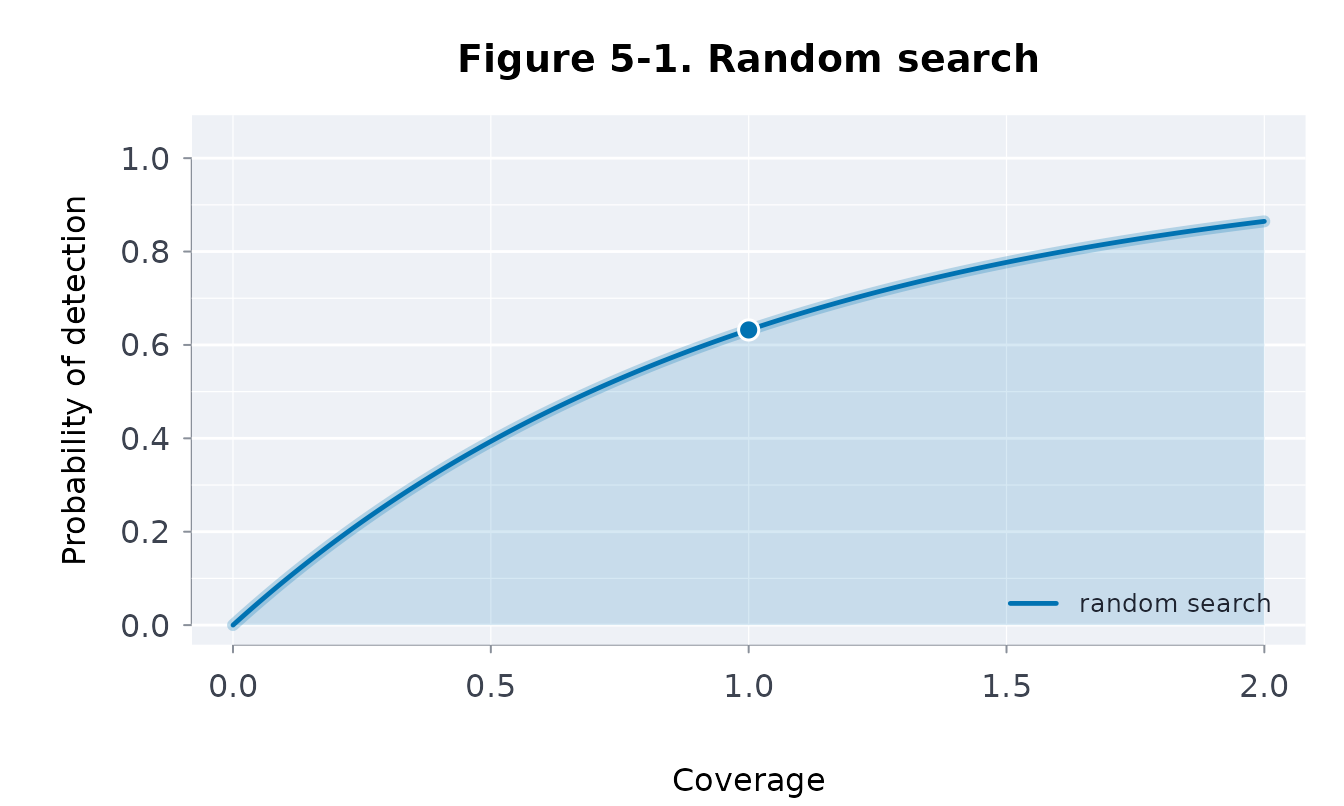
Figures 5-2 to 5-5. A parallel sweep at track
spacing S has coverage C = W / S. With a
definite range sensor the POD is min(C, 1): half the gap is
seen at S = 2W, all of it at S = W.
srchfig("5-2")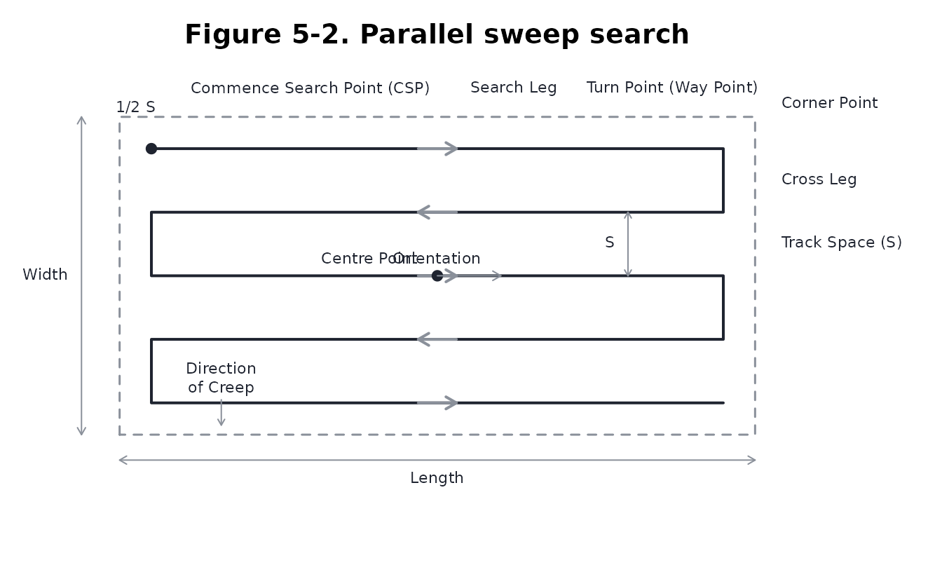
srchfig("5-3")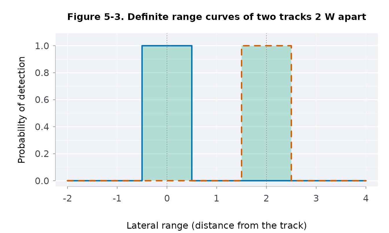
srchfig("5-4")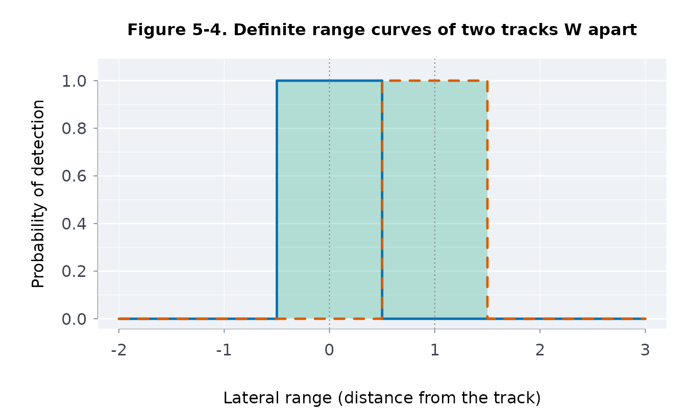
srchfig("5-5")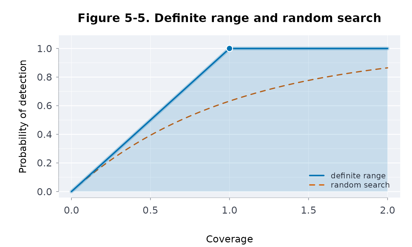
Figures 5-6 and 5-7. M-Beta curves overlap once the
tracks are closer than their width: POD = C below
C = M and 1 - (1 - M)^(C / M) above it, 0.75
and 0.6836 at coverage 1 for M = 0.5 and
M = 0.25, nearer the random search curve as M
falls.
srchfig("5-6")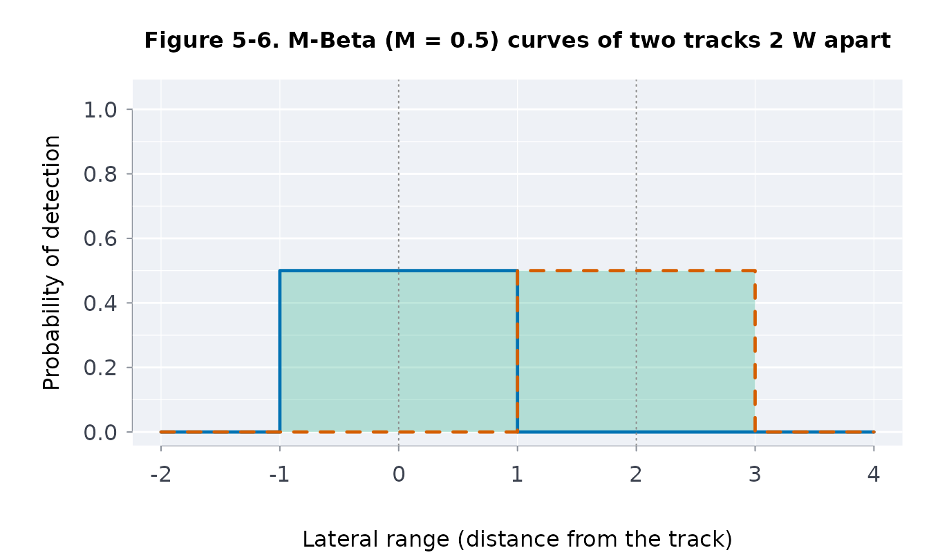
srchfig("5-7")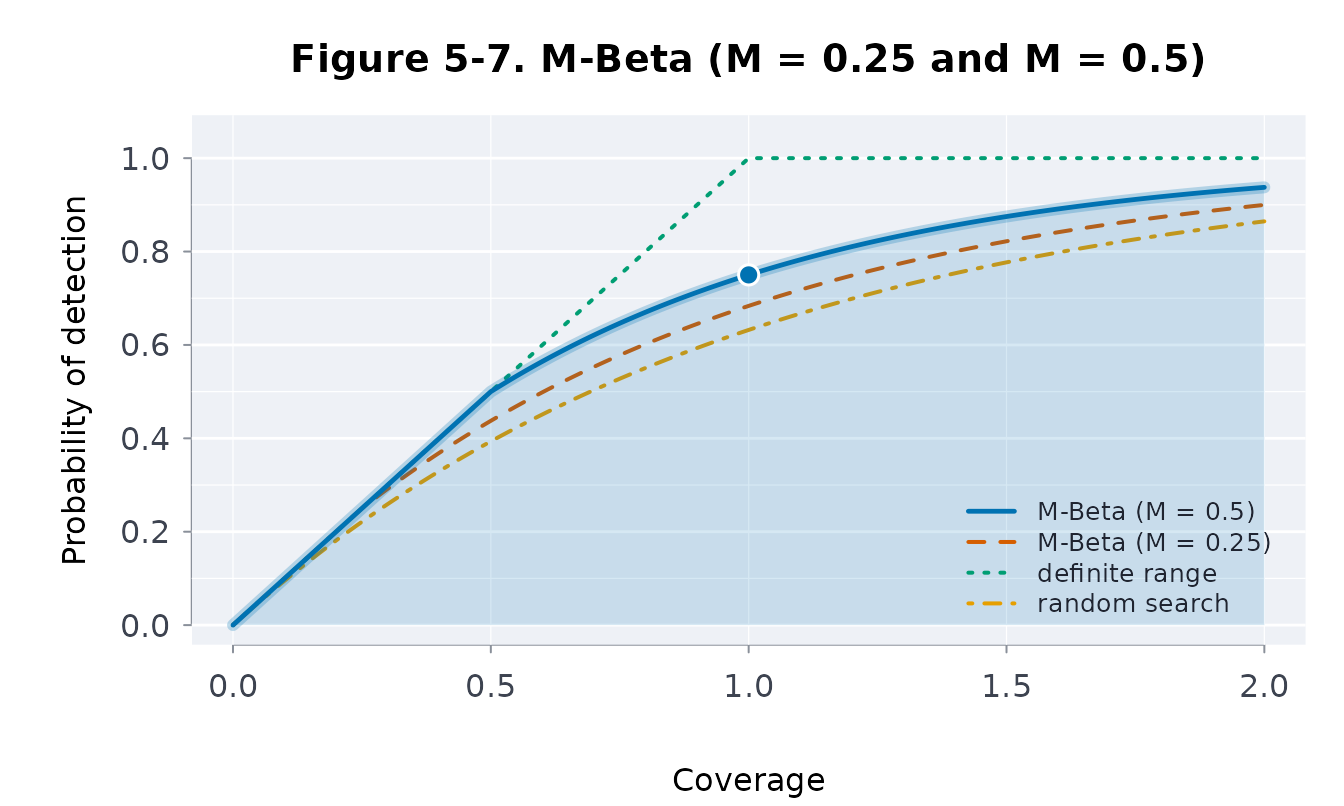
srchpod(c(0.5, 1, 2), "mbeta", m = 0.25)
#> ╭── Probability of detection ─────────────────────────────────────────╮
#> │   Model      M-Beta                                                 │
#> │   M          0.25                                                   │
#> │   Coverages  3                                                      │
#> │                                                                     │
#> │   coverage       pod                                                │
#> │   --------  --------                                                │
#> │    0.50000  0.437500                                                │
#> │    1.00000  0.683594                                                │
#> │    2.00000  0.899887                                                │
#> │                                                                     │
#> │   M-Beta model, M = 0.25                                            │
#> │   Coverage is effort over area (sweep width x track length / area); │
#> │   pod is the chance a search at that coverage finds the object.     │
#> ╰─────────────────────────────────────────────────────────────────────╯
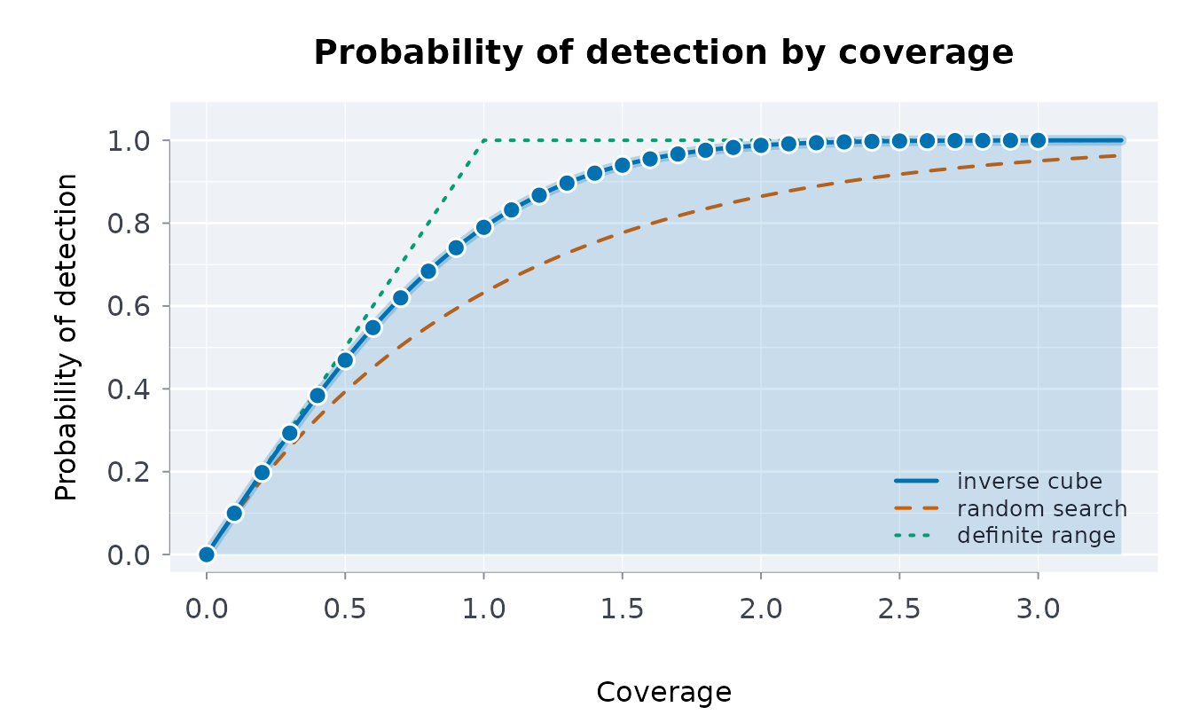
Figure 5-8. The inverse cube parallel sweep gives
POD = erf(sqrt(pi) C / 2), 0.7899 at coverage 1, between
the definite range and random search curves. pswppod()
computes the same sweep directly, for any curve.
srchfig("5-8")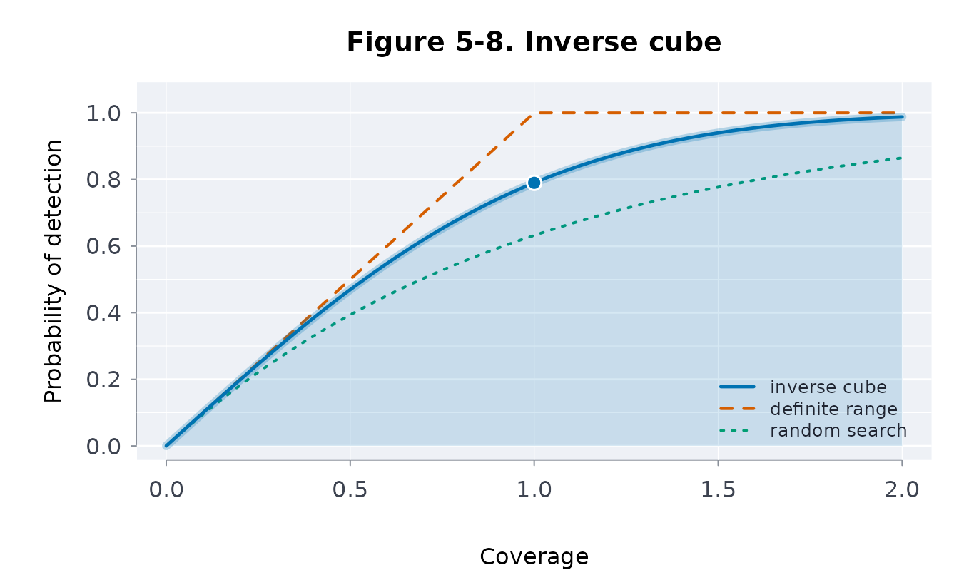
pswppod(W = 1, S = 1)
#> [1] 0.7899086
Figure 5-9. Poorer conditions shrink the sweep
width, and a cross-track navigation error of standard deviation
sigma flattens the curve: the expected curve is the
convolution phi(x) = integral of p(x - t) Z(t, sigma) dt,
whose area is still W
(ltrlrng(..., navsd = )). The plate is blank in the
published file; it is drawn from the text.
srchfig("5-9")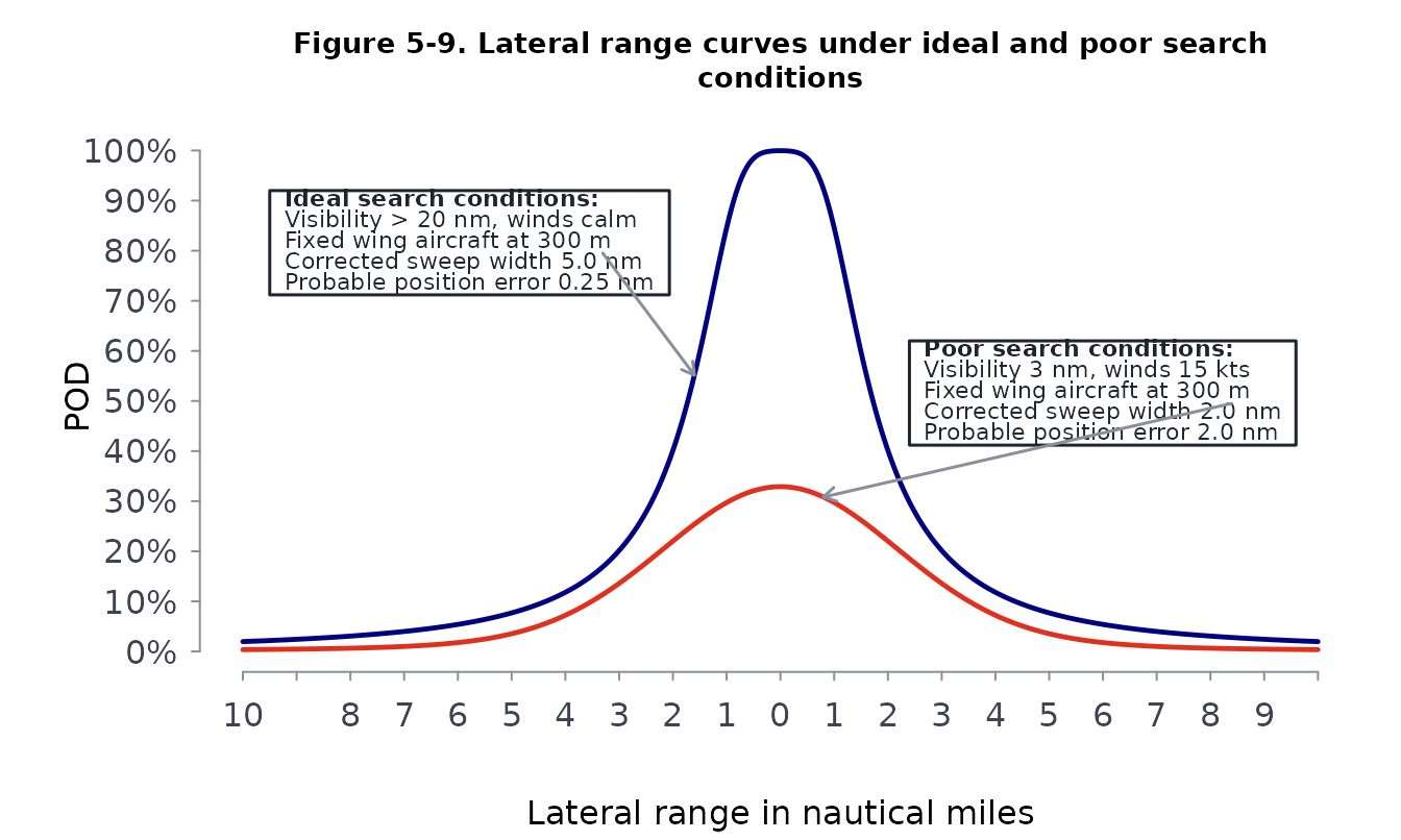
Optimal search
Figures 6-1 and 6-2. With half the probability in a 3 by 3 square inside a 5 by 5 one and effort for half the area, the trial squares of the whole area, half of it and a third of it hold 100%, 60.94% and 46.30%; at coverage 1 the middle trial succeeds most often.
srchfig("6-1")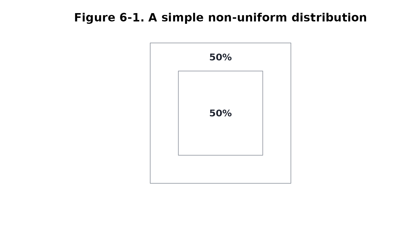
srchfig("6-2")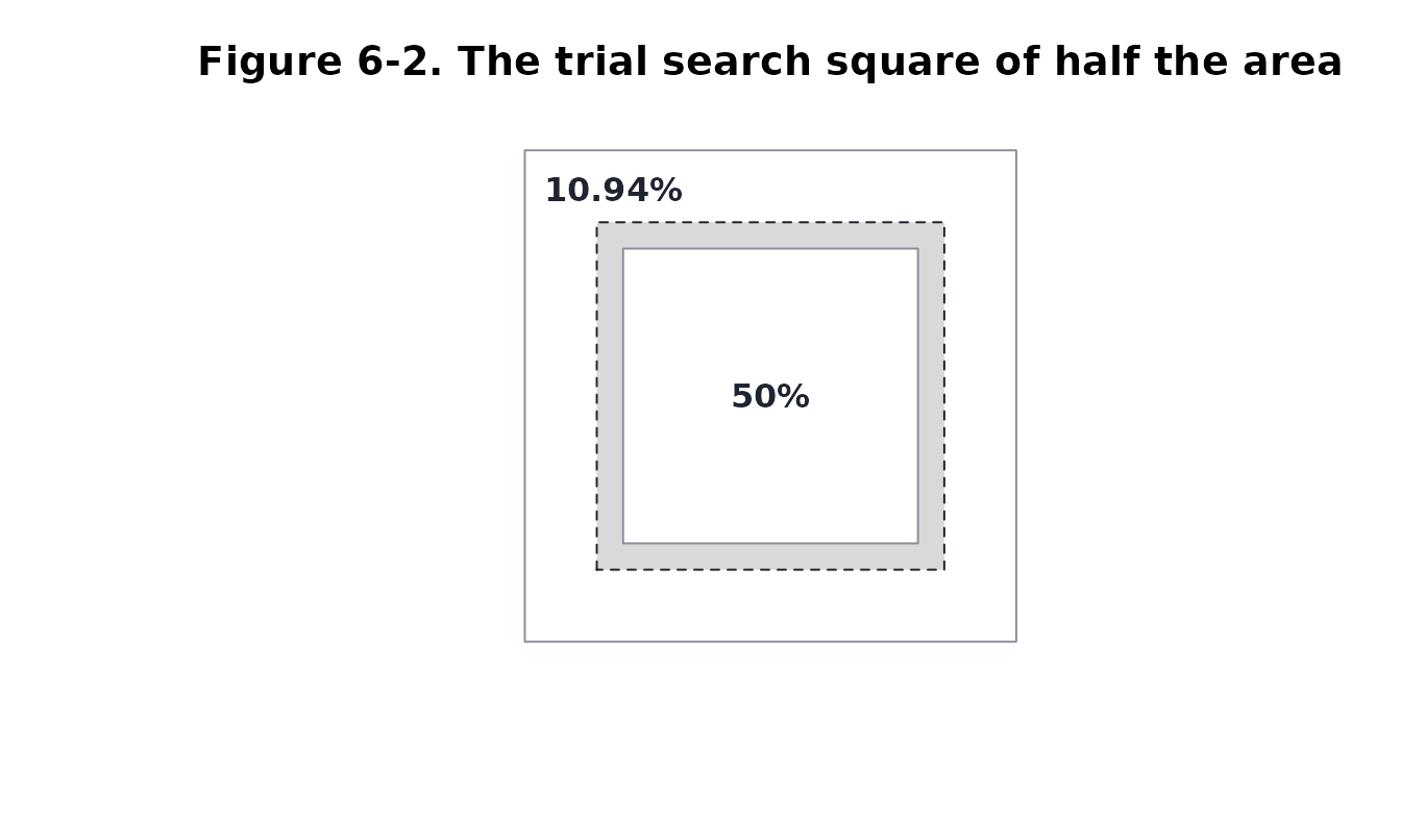
Figures 6-3 and 6-4. For a point datum,
optsqr() finds the square that an effort, spread evenly,
should cover: the search factor is its half side in units of
E. An effort of 4 E^2 gives a factor of 1.02,
coverage 0.96 and POS 0.4578, as the book’s program found.
optsqr(4)
#> ╭── Optimal square searches ────────────────────────────────────────────────╮
#> │   Searches                 1                                              │
#> │   Total effort             4                                              │
#> │   Chance found by the end  0.4578                                         │
#> │                                                                           │
#> │   search  effort  releff  cumeff  factor   side     poc  coverage     pod │
#> │   ------  ------  ------  ------  ------  -----  ------  --------  ------ │
#> │        1       4       4       4   1.021  2.042  0.5940    0.9592  0.7707 │
#> │                                                                           │
#> │   search     pos  cumpos                                                  │
#> │   ------  ------  ------                                                  │
#> │        1  0.4578  0.4578                                                  │
#> │                                                                           │
#> │   Each search covers the square (of side 'side') that gives it the best   │
#> │   chance of success after the searches before it. poc is the chance the   │
#> │   object is in that square, pod the chance of detecting it there, pos     │
#> │   their product and cumpos the running chance it has been found.          │
#> ╰───────────────────────────────────────────────────────────────────────────╯
srchfig("6-3")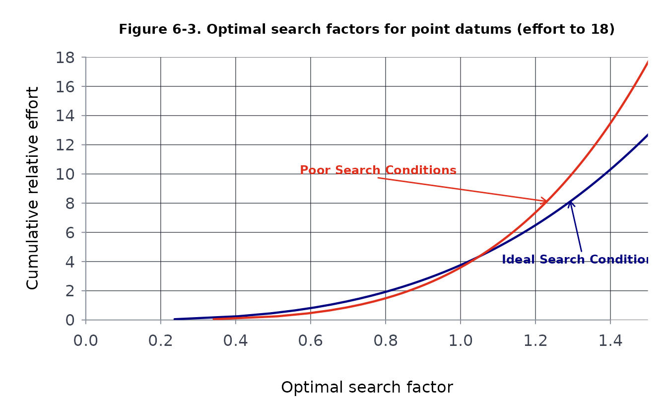
srchfig("6-4")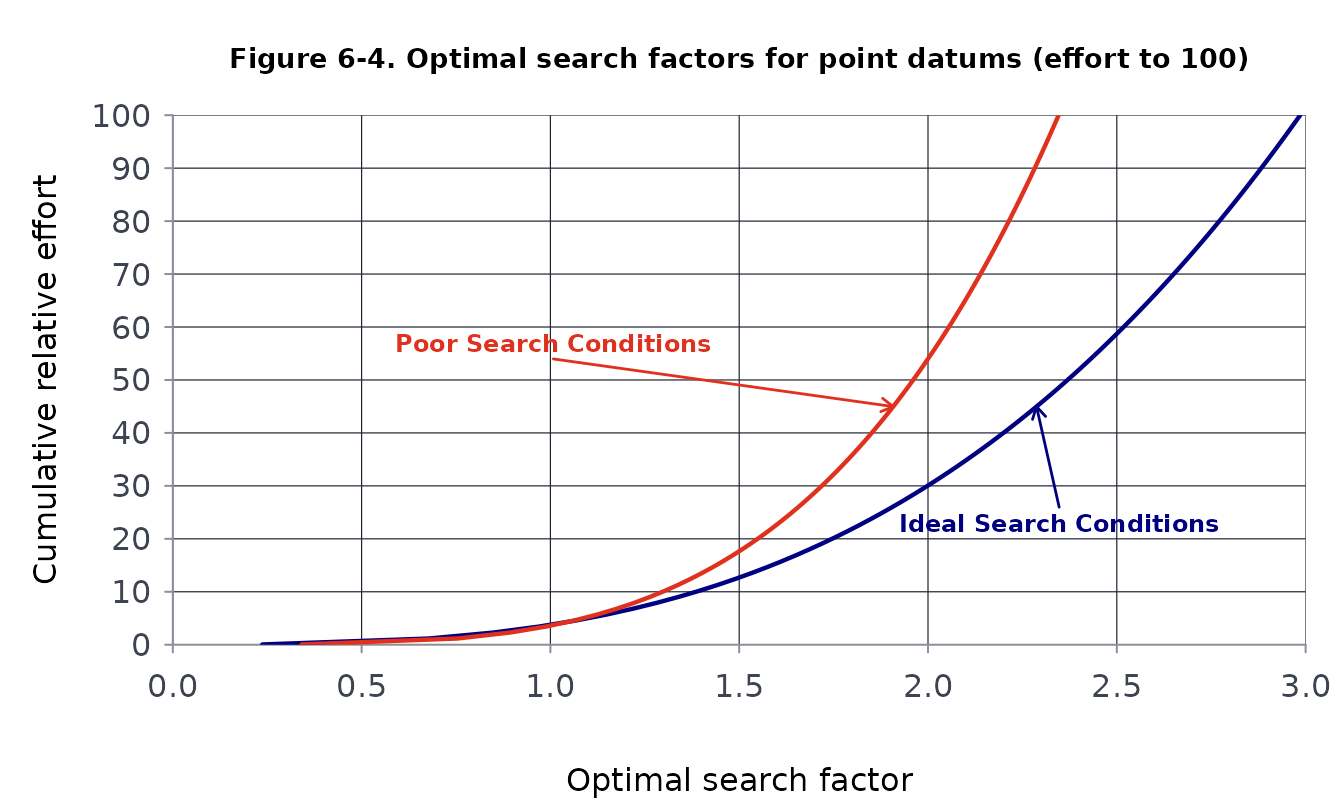
Figure 6-5. By the additive principle, a series of searches each optimal for what the earlier ones left does as well as one optimal search with all the effort: the cumulative probability of success depends on the cumulative effort.
srchfig("6-5")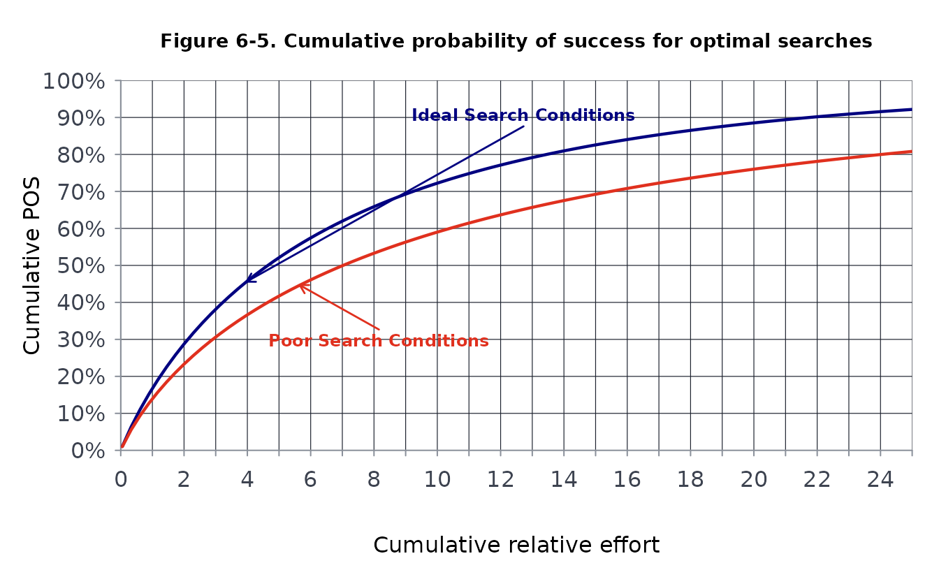
Figure 6-6. Searching in a series with random
efforts between 0.1 and 50 E^2, the optimal factors cluster
around the curve, except where a much smaller effort follows a large one
and the best use of it is the remaining central peak.
srchfig("6-6")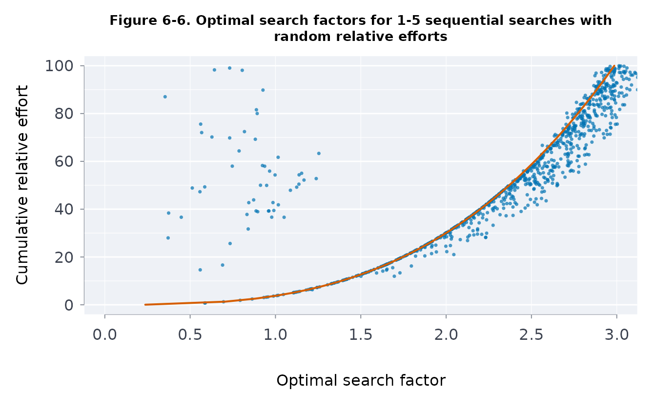
Your own search
The figures use the book’s numbers; every function takes yours, and
each result has a plot() method. srchfig()
lists, for each of the 36 figures, the one line that draws it from your
own numbers (replace the example inputs; a schematic gives the
computation it pictures):
# an HTML table with each line in <code>: in a Markdown table a `$` starts a
# formula and a `|` ends the cell, so both are written as entities
tab <- srchfig()[, c("fig", "caption", "yours")]
esc <- function(x) {
for (r in list(
c("&", "&"),
c("<", "<"),
c(">", ">"),
c("$", "$"),
c("|", "|")
)) {
x <- gsub(r[1], r[2], x, fixed = TRUE)
}
x
}
tab$caption <- esc(tab$caption)
tab$yours <- sprintf("<code>%s</code>", esc(tab$yours))
knitr::kable(
tab,
format = "html",
escape = FALSE,
row.names = FALSE,
col.names = c("Figure", "Caption", "From your own numbers")
)| Figure | Caption | From your own numbers |
|---|---|---|
| 3-1 | Probability density distribution for a point datum with top view |
plot(datumpmap(seq(-4, 4, by = 0.25), seq(-4, 4, by = 0.25),
center = c(0, 0), sigma = 1.5), view = “both”)
|
| 3-2 | Circle of radius one standard deviation and its circumscribed square |
sum(datumpmap(c(-1.5, 1.5), c(-1.5, 1.5), sigma = 1.5)$poc)
|
| 3-3 | Circle of radius E and its circumscribed square |
sum(datumpmap(c(-1, 1) * 1.177 * 1.5, c(-1, 1) * 1.177 * 1.5,
sigma = 1.5)$poc)
|
| 3-4 | Probability map for a point datum |
plot(datumpmap(c(-3, -1, 1, 3) * 1.77, c(-3, -1, 1, 3) * 1.77,
sigma = 1.5), view = “cells”)
|
| 3-5 | Circle of radius 1.1 E and its circumscribed square |
sum(datumpmap(c(-1, 1) * 1.295 * 1.5, c(-1, 1) * 1.295 * 1.5,
sigma = 1.5)$poc)
|
| 3-6 | Line datum: circles at the end points boxed in |
plot(datumpmap(seq(-4, 4, by = 0.25), seq(-4, 4, by = 0.25),
“line”, center = c(0, -2), end = c(0, 2), sigma = 1), view =
“both”)
|
| 3-7 | Probability density distribution for a line datum connecting two point datums |
plot(datumpmap(seq(-4, 4, by = 0.25), seq(-4, 4, by = 0.25),
“line”, center = c(0, -2), end = c(0, 2), sigma = 1), view =
“both”)
|
| 3-8 | Probability density distribution for a line datum with top view |
plot(datumpmap(seq(-4, 4, by = 0.25), seq(-4, 4, by = 0.25),
“corridor”, center = c(0, -2), end = c(0, 2), sigma = 1), view =
“both”)
|
| 3-9 | Strip of width 2 E centred on the datum line |
plot(datumpmap(c(-5, 5), c(-1.18, 1.18), “corridor”, center =
c(-4, 0), end = c(4, 0), sigma = 1), view = “cells”)
|
| 3-10 | Example of a completed probability map for a line datum |
plot(datumpmap(0:10, c(-3, -1.8, -0.6, 0.6, 1.8, 3), “corridor”,
center = c(0, 0), end = c(10, 0), sigma = 1), view = “cells”)
|
| 3-11 | Uniform probability density distribution with top view |
plot(datumpmap(seq(-4, 4, by = 0.25), seq(-4, 4, by = 0.25),
“area”, center = c(-2, -1.5), end = c(2, 1.5)), view = “both”)
|
| 3-12 | Probability map for an area datum |
plot(datumpmap(0:5, 0:4, “area”, center = c(0, 0), end = c(5, 4)),
view = “cells”)
|
| 3-13 | Generalized probability density distribution with top view |
plot(datumpmap(0:5, 0:4, “general”, wts = matrix(c(1:10, 10:1), 4,
5)), view = “both”)
|
| 3-14 | Probability map for a generalized datum |
plot(datumpmap(0:5, 0:4, “general”, wts = matrix(c(1:10, 10:1), 4,
5)), view = “cells”)
|
| 4-1 | Lateral range curves: definite range, M-Beta, inverse cube and another sensor |
plot(ltrlrng(seq(-3, 3, by = 0.05), W = 0.8, model = “mbeta”, m =
0.5))
|
| 4-2 | Definite range lateral range curve |
plot(ltrlrng(seq(-3, 3, by = 0.05), W = 0.8, model =
“definite”))
|
| 4-3 | The area swept by a definite range sensor |
plot(ltrlrng(seq(-3, 3, by = 0.05), W = 0.8, model = “definite”),
equiv = TRUE)
|
| 4-4 | M-Beta lateral range curve, M = 0.5 |
plot(ltrlrng(seq(-3, 3, by = 0.05), W = 0.8, model = “mbeta”, m =
0.5), equiv = TRUE)
|
| 4-5 | M-Beta lateral range curve, M = 0.25 |
plot(ltrlrng(seq(-3, 3, by = 0.05), W = 0.8, model = “mbeta”, m =
0.25), equiv = TRUE)
|
| 4-6 | The geometry of the inverse cube law |
plot(ltrlrng(seq(-3, 3, by = 0.05), W = 0.8, model =
“invcube”))
|
| 4-7 | Inverse cube lateral range curve and its sweep width |
plot(ltrlrng(seq(-3, 3, by = 0.05), W = 0.8, model = “invcube”),
equiv = TRUE)
|
| 5-1 | Random search |
plot(srchpod(seq(0, 3, by = 0.1), model = “random”))
|
| 5-2 | Parallel sweep search |
pswppod(W = 0.8, S = 1, model = “invcube”)
|
| 5-3 | Definite range curves of two tracks 2 W apart |
plot(ltrlrng(seq(-3, 3, by = 0.05), W = 0.8, model = “definite”),
spacing = 1.6)
|
| 5-4 | Definite range curves of two tracks W apart |
plot(ltrlrng(seq(-3, 3, by = 0.05), W = 0.8, model = “definite”),
spacing = 0.8)
|
| 5-5 | Definite range and random search |
plot(srchpod(seq(0, 3, by = 0.1), “definite”), models =
c(“definite”, “random”))
|
| 5-6 | M-Beta (M = 0.5) curves of two tracks 2 W apart |
plot(ltrlrng(seq(-3, 3, by = 0.05), W = 0.8, model = “mbeta”, m =
0.5), spacing = 1.6)
|
| 5-7 | M-Beta (M = 0.25 and M = 0.5) |
plot(srchpod(seq(0, 3, by = 0.1), “mbeta”, m = 0.5), models =
c(“mbeta”, “definite”, “random”), m = c(0.5, 0.25))
|
| 5-8 | Inverse cube |
plot(srchpod(seq(0, 3, by = 0.1), “invcube”), models =
c(“invcube”, “definite”, “random”))
|
| 5-9 | Lateral range curves under ideal and poor search conditions |
plot(ltrlrng(seq(-3, 3, by = 0.05), W = 0.8, model = “invcube”,
navsd = 0.3), spacing = 1)
|
| 6-1 | A simple non-uniform distribution |
optsqr(effort = 2)
|
| 6-2 | The trial search square of half the area |
optsqr(effort = 2)$side
|
| 6-3 | Optimal search factors for point datums (effort to 18) |
with(do.call(rbind, lapply(seq(0.5, 18, by = 0.5), optsqr)),
plot(factor, cumeff, type = “l”))
|
| 6-4 | Optimal search factors for point datums (effort to 100) |
with(do.call(rbind, lapply(seq(2, 100, by = 2), optsqr)),
plot(factor, cumeff, type = “l”))
|
| 6-5 | Cumulative probability of success for optimal searches |
with(do.call(rbind, lapply(seq(0.5, 25, by = 0.5), optsqr)),
plot(cumeff, 100 * cumpos, type = “l”))
|
| 6-6 | Optimal search factors for 1-5 sequential searches with random relative efforts |
optsqr(c(1, 0.5, 2, 1.5))
|
The most used of them, step by step. Say a sensor’s sweep width is 0.8 nautical miles and its detection falls off as the inverse cube of the lateral range. Its lateral range curve, and the picture of what the sweep width means (the objects missed inside it equal those seen outside it, Figure 4-7):
plot(lr, equiv = TRUE)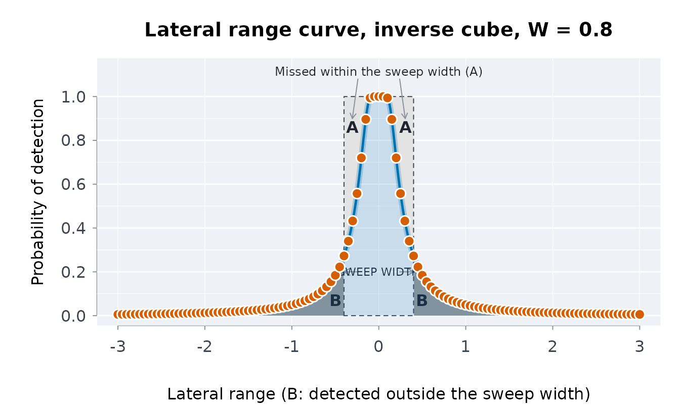
A sweep width can also come from a field trial: the share of objects
detected at each lateral range, measured on both sides of the track.
swpwdth() integrates the curve.
d <- c(-3, -2, -1.5, -1, -0.5, -0.25, 0, 0.25, 0.5, 1, 1.5, 2, 3)
p <- c(0.01, 0.08, 0.2, 0.45, 0.75, 0.9, 0.95, 0.9, 0.75, 0.45, 0.2, 0.08, 0.01)
swpwdth(d, p)
#> [1] 2.03
The probability of detection for the coverage a plan gives (coverage is sweep width times track length over the area), and for parallel sweeps at a track spacing of 1 with a navigation error of 0.1:
pswppod(W = 0.8, S = 1, navsd = 0.1)
#> [1] 0.6806056
After a search of three areas that found nothing, the chance the object is in each area is updated by what each search could have detected:
srchscs(poc = c(0.5, 0.3, 0.2), pod = c(0.8, 0.5, 0))
#> ╭── Probability of success ────────────────────────────────────────────╮
#> │   Areas        3                                                     │
#> │   Searches     1                                                     │
#> │   Overall POS  0.55                                                  │
#> │                                                                      │
#> │   area     poc  cumpod  posarea  pocupd                              │
#> │   ----  ------  ------  -------  ------                              │
#> │      1  0.5000  0.8000   0.4000  0.2222                              │
#> │      2  0.3000  0.5000   0.1500  0.3333                              │
#> │      3  0.2000  0.0000   0.0000  0.4444                              │
#> │                                                                      │
#> │   POS 0.55 after 1 search                                            │
#> │   poc: chance the object is in the area; cumpod: chance the searches │
#> │   detect it there; pocupd: the poc after the searches found nothing. │
#> ╰──────────────────────────────────────────────────────────────────────╯
Your own search, step by step
The same functions plan a real search from your own numbers, one call per step. Use one distance unit throughout (kilometres here; nautical miles at sea): the grid, the positions, the sweep width and the track length are all in it, and areas in its square.
1. The search area and its grid. A hiker is overdue;
the last known position (LKP) is 2 km east and 3 km north of the base.
Lay a grid of cells over the area you could search: here 12 km by 12 km
in half-kilometre cells. xedg and yedg are the
cell edges, west to east and south to north; cells need not be
equal.
2. The probability map. datumpmap()
puts the chance the hiker is in each cell on the grid. For a point datum
give the LKP as center and the position error as
sigma, one standard deviation (about 1.5 km, from the time
and terrain since the LKP). A route between two points is
datum = "line" or "corridor" with
end, a region known only by its bounds
datum = "area", and a map of your own (cell shares from the
planners’ scenarios, say) is datum = "general" with
wts, one row per y cell and one column per
x cell.
m <- datumpmap(xe, ye, center = c(2, 3), sigma = 1.5)
m
#> ╭── Datum probability map (point datum) ──────────────────────────────────╮
#> │   Datum   point                                                         │
#> │   Centre  2, 3                                                          │
#> │   Sigma   1.5                                                           │
#> │   Grid    24 x 24 cells (x by y)                                        │
#> │                                                                         │
#> │   The most likely cells                                                 │
#> │       x      y      poc                                                 │
#> │   -----  -----  -------                                                 │
#> │   1.750  2.750  0.01705                                                 │
#> │   1.750  3.250  0.01705                                                 │
#> │   2.250  2.750  0.01705                                                 │
#> │   2.250  3.250  0.01705                                                 │
#> │   1.250  2.750  0.01527                                                 │
#> │                                                                         │
#> │   24 x 24 cells (x by y); 0.0% of the probability lies outside the grid │
#> ╰─────────────────────────────────────────────────────────────────────────╯
plot(m)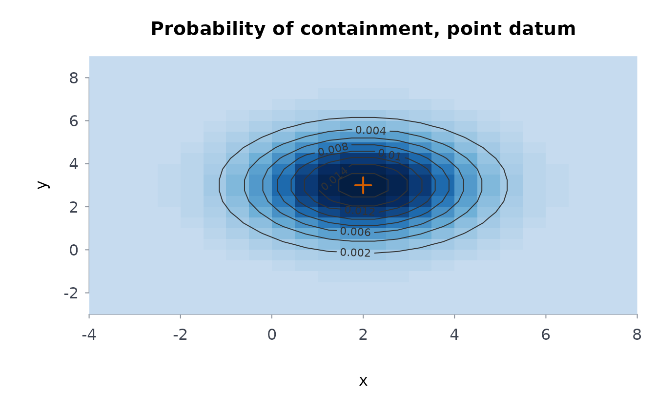
Two scenarios weighted by the planners (70% on the LKP, 30% that the hiker took the trail to the north-east) are mixed cell by cell, and the mixture is a general datum (its weights are scaled to sum to 1 over the grid):
trail <- datumpmap(xe, ye, "corridor", c(2, 3), sigma = 0.5, end = c(2, 8))
mix <- datumpmap(xe, ye, "general", wts = 0.7 * m$poc + 0.3 * trail$poc)
plot(mix)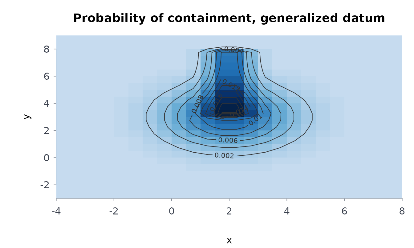
3. The sweep width and the detection model. The
sweep width W comes from a published table for the sensor,
the object and the conditions, or from a field trial of your own with
swpwdth() (above). The detection model says how detection
falls off with distance: "invcube" for good conditions and
evenly spaced tracks, "random" for poor conditions or
uneven tracks (the conservative choice), "definite" for a
sensor that sees everything within W / 2. Here the ground
teams’ sweep width is 0.6 km.
4. Effort, and the probability of detection. The
effort is the track length walked in each cell. Say today’s teams walked
2 km of track in each of the four cells round the LKP.
srchpod() with W, effort and
area turns that into the coverage and the POD of each cell;
area = m takes the map’s cell areas, and
effort is laid out like the map (one row per y
cell):
walked <- matrix(0, nrow(m$poc), ncol(m$poc))
walked[12:13, 12:13] <- 2
pd <- srchpod(W = 0.6, effort = walked, area = m, model = "random")
range(pd)
#> [1] 0.0000000 0.9917703
5. The probability of success, and the map after a search
that found nothing. srchscs() takes the map and
the PODs: pos is the chance today’s search found the hiker,
and map the probability map updated by what was searched
(cells searched hard become less likely, the rest more likely):
day1 <- srchscs(m, pd)
day1
#> ╭── Probability of success ────────────────────────────────────────────╮
#> │   Areas        576                                                   │
#> │   Searches     1                                                     │
#> │   Overall POS  0.06762                                               │
#> │   Map          24 x 24 cells (x by y), updated in $map               │
#> │                                                                      │
#> │   area      poc  cumpod  posarea   pocupd                            │
#> │   ----  -------  ------  -------  -------                            │
#> │    276  0.01705  0.9918  0.01691  0.00015                            │
#> │    277  0.01705  0.9918  0.01691  0.00015                            │
#> │    300  0.01705  0.9918  0.01691  0.00015                            │
#> │    301  0.01705  0.9918  0.01691  0.00015                            │
#> │    252  0.01527  0.0000  0.00000  0.01638                            │
#> │    253  0.01527  0.0000  0.00000  0.01638                            │
#> │    275  0.01527  0.0000  0.00000  0.01638                            │
#> │    278  0.01527  0.0000  0.00000  0.01638                            │
#> │    299  0.01527  0.0000  0.00000  0.01638                            │
#> │    302  0.01527  0.0000  0.00000  0.01638                            │
#> │    324  0.01527  0.0000  0.00000  0.01638                            │
#> │    325  0.01527  0.0000  0.00000  0.01638                            │
#> │    251  0.01368  0.0000  0.00000  0.01467                            │
#> │    254  0.01368  0.0000  0.00000  0.01467                            │
#> │    323  0.01368  0.0000  0.00000  0.01467                            │
#> │    326  0.01368  0.0000  0.00000  0.01467                            │
#> │    228  0.01225  0.0000  0.00000  0.01314                            │
#> │    229  0.01225  0.0000  0.00000  0.01314                            │
#> │    274  0.01225  0.0000  0.00000  0.01314                            │
#> │    298  0.01225  0.0000  0.00000  0.01314                            │
#> │                                                                      │
#> │   POS 0.06762 after 1 search                                         │
#> │   poc: chance the object is in the area; cumpod: chance the searches │
#> │   detect it there; pocupd: the poc after the searches found nothing. │
#> │                                                                      │
#> │   The 20 most likely of 576 cells.                                   │
#> ╰──────────────────────────────────────────────────────────────────────╯
plot(day1$map)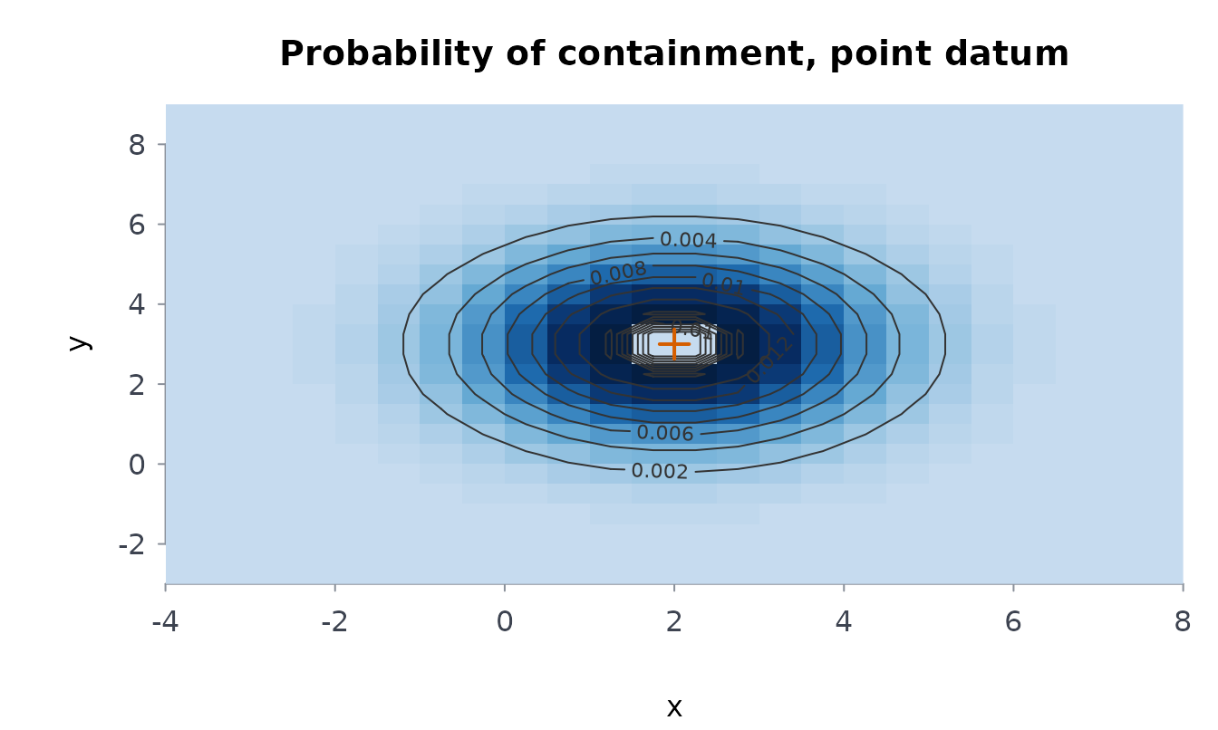
6. Plan the next search. opteffort()
spreads tomorrow’s 40 km of track over the updated map to make the
chance of finding the hiker as large as possible (Stone 1975), under
random search detection. Its result goes straight back into
srchscs() for the day after:
day2 <- opteffort(day1$map, W = 0.6, effort = 40)
day2
#> ╭── Optimal allocation of effort ─────────────────────────────╮
#> │   Total effort    40                                        │
#> │   Sweep width W   0.6                                       │
#> │   Cells searched  108 of 576                                │
#> │   POS             0.5467                                    │
#> │                                                             │
#> │   cell      poc  effort  coverage     pod                   │
#> │   ----  -------  ------  --------  ------                   │
#> │    252  0.01638  0.7356     1.766  0.8289                   │
#> │    253  0.01638  0.7356     1.766  0.8289                   │
#> │    275  0.01638  0.7356     1.766  0.8289                   │
#> │    278  0.01638  0.7356     1.766  0.8289                   │
#> │    299  0.01638  0.7356     1.766  0.8289                   │
#> │    302  0.01638  0.7356     1.766  0.8289                   │
#> │    324  0.01638  0.7356     1.766  0.8289                   │
#> │    325  0.01638  0.7356     1.766  0.8289                   │
#> │    251  0.01467  0.6898     1.655  0.8090                   │
#> │    254  0.01467  0.6898     1.655  0.8090                   │
#> │    323  0.01467  0.6898     1.655  0.8090                   │
#> │    326  0.01467  0.6898     1.655  0.8090                   │
#> │    228  0.01314  0.6439     1.545  0.7868                   │
#> │    229  0.01314  0.6439     1.545  0.7868                   │
#> │    274  0.01314  0.6439     1.545  0.7868                   │
#> │    298  0.01314  0.6439     1.545  0.7868                   │
#> │    279  0.01314  0.6439     1.545  0.7868                   │
#> │    303  0.01314  0.6439     1.545  0.7868                   │
#> │    348  0.01314  0.6439     1.545  0.7868                   │
#> │    349  0.01314  0.6439     1.545  0.7868                   │
#> │                                                             │
#> │   POS 0.5467 from effort 40 over 108 of 576 cells (W = 0.6) │
#> │                                                             │
#> │   ... and 88 more cells                                     │
#> ╰─────────────────────────────────────────────────────────────╯
day3 <- srchscs(day1$map, day2)
day3$pos
#> [1] 0.546653
7. Plot. Every result has a plot()
method: the allocation as a map of the effort in each cell, the map as
an image, a surface or its cells with their percentages.
plot(day2)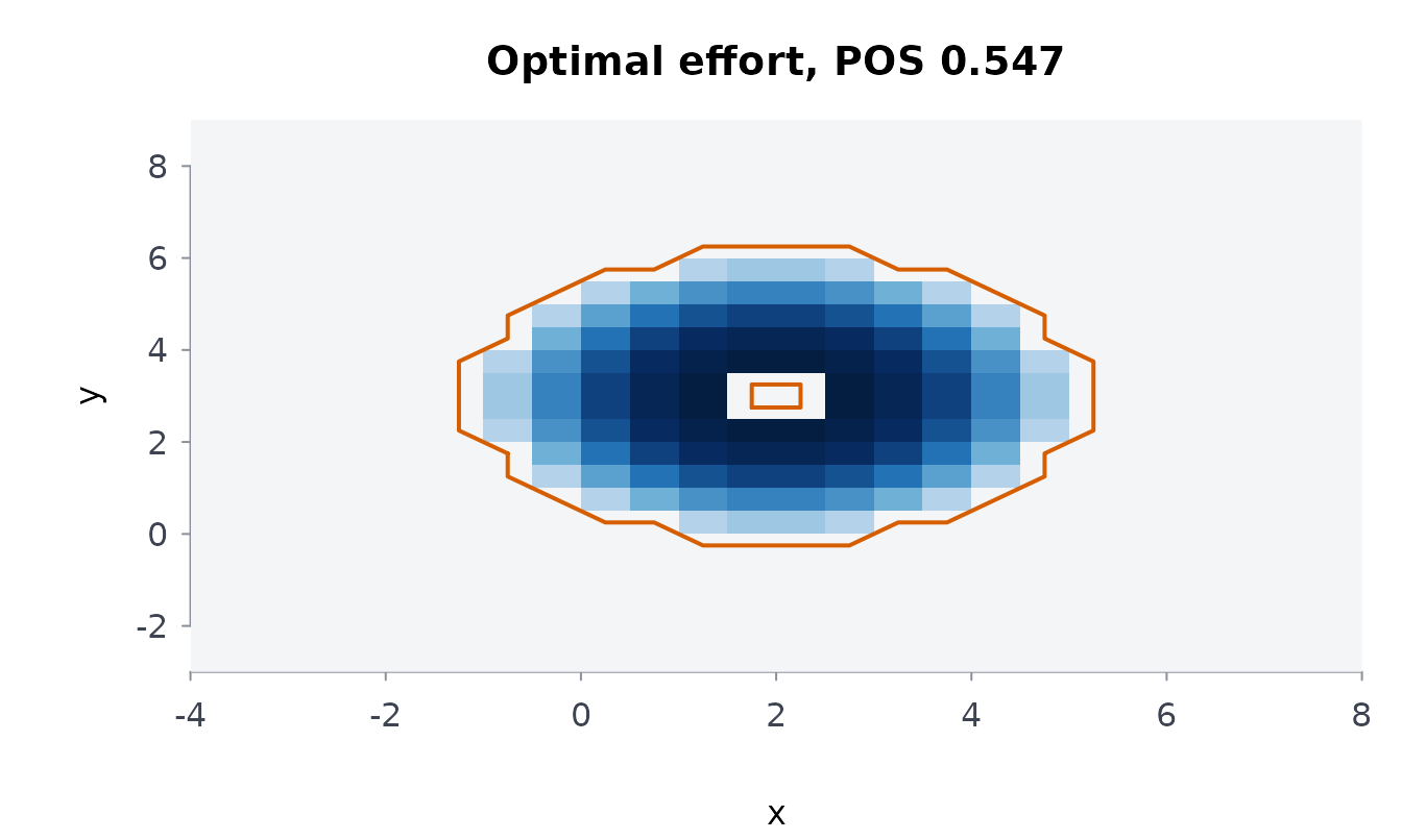
plot(day1$map, view = "both")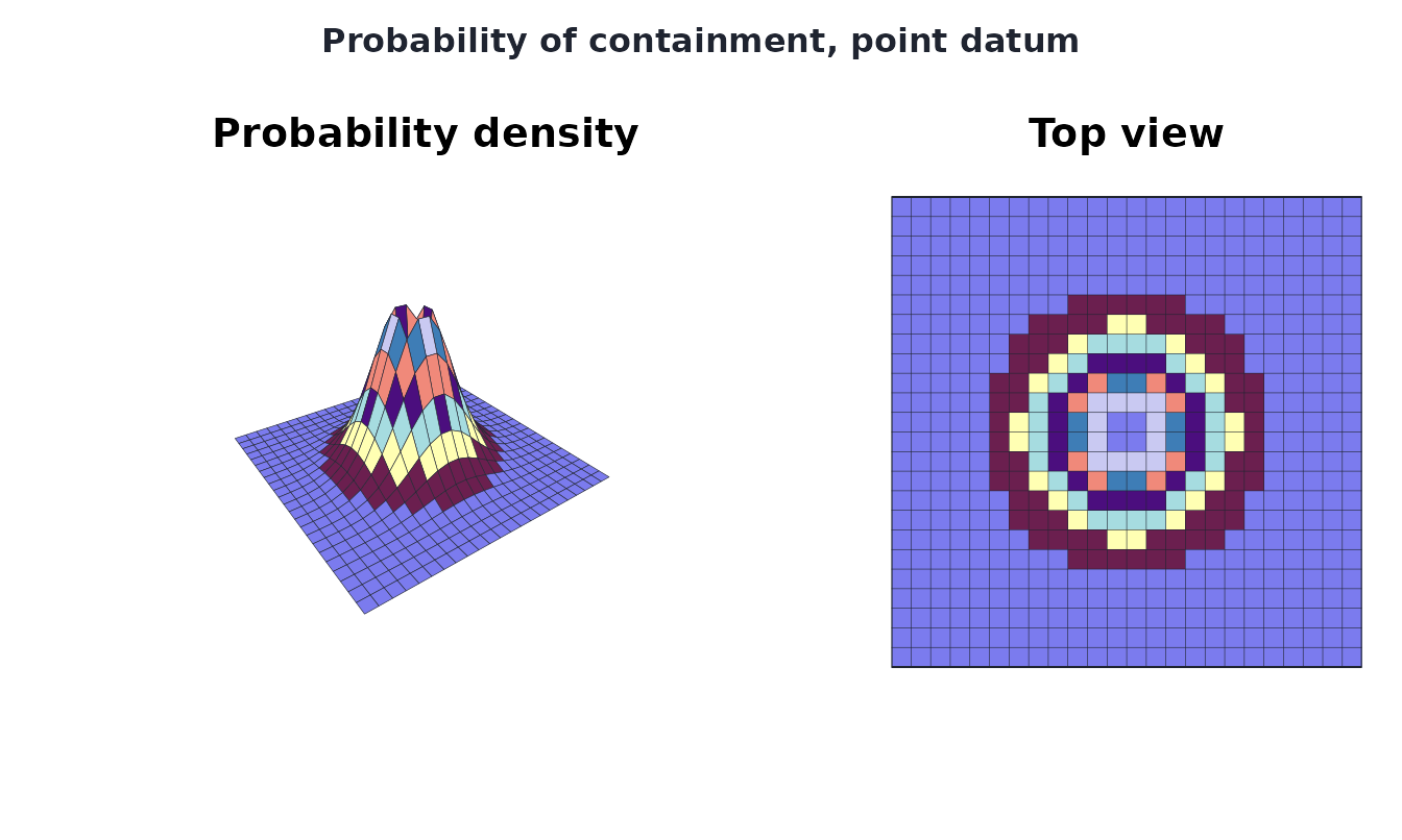
For a single point datum with no grid, optcrcsrch()
gives Koopman’s optimal circle directly, and optsqr() the
optimal square, search after search:
optcrcsrch(sigma = 1.5, W = 0.6, effort = 40)
#> ╭── Optimal search of a circular normal datum ────────────────────────╮
#> │   sigma    1.5                                                      │
#> │   W        0.6                                                      │
#> │   effort   40                                                       │
#> │   radius   2.88                                                     │
#> │   pos      0.5497                                                   │
#> │   cntrdns  3.071                                                    │
#> │                                                                     │
#> │   Spread the effort evenly over a circle of radius 2.88: the chance │
#> │   of finding the object is then 55.0%.                              │
#> │                                                                     │
#> │   cntrdns: the coverage at the centre of the circle.                │
#> ╰─────────────────────────────────────────────────────────────────────╯
optsqr(c(40, 40) * 0.6, E = 1.1774 * 1.5)
#> ╭── Optimal square searches ────────────────────────────────────────────────╮
#> │   Searches                 2                                              │
#> │   Total effort             48                                             │
#> │   Chance found by the end  0.8047                                         │
#> │                                                                           │
#> │   search  effort  releff  cumeff  factor   side     poc  coverage     pod │
#> │   ------  ------  ------  ------  ------  -----  ------  --------  ------ │
#> │        1      24   7.695    7.69   1.270  4.485  0.7484    1.1929  0.8651 │
#> │        2      24   7.695   15.39   1.696  5.991  0.7460    0.6686  0.5980 │
#> │                                                                           │
#> │   search     pos  cumpos                                                  │
#> │   ------  ------  ------                                                  │
#> │        1  0.6475  0.6475                                                  │
#> │        2  0.4461  0.8047                                                  │
#> │                                                                           │
#> │   Each search covers the square (of side 'side') that gives it the best   │
#> │   chance of success after the searches before it. poc is the chance the   │
#> │   object is in that square, pod the chance of detecting it there, pos     │
#> │   their product and cumpos the running chance it has been found.          │
#> ╰───────────────────────────────────────────────────────────────────────────╯
References
Frost, J. R. (1996). The Theory of Search: A Simplified Explanation. Soza and Company and U.S. Coast Guard Office of Search and Rescue. Chapters 3-6 and their figures.
Koopman, B. O. (1946). Search and Screening. OEG Report 56, Office of the Chief of Naval Operations.
Koopman, B. O. (1956-1957). The theory of search, parts I-III. Operations Research 4(3), 324-346; 4(5), 503-531; 5(5), 613-626.
Stone, L. D. (1975). Theory of Optimal Search. Academic Press.